Linear Function Approximation

A probability distribution representation is used to describe return functions

in terms of a collection of numbers that can be stored in a computer’s mem-

ory. With it, we can devise algorithms that operate on return distributions in a

computationally eﬃcient manner, including distributional dynamic program-

ming algorithms and incremental algorithms such as CTD and QTD. Function

approximation arises when our representation of the value or return function

uses parameters that are shared across states. This allows reinforcement learning

methods to be applied to domains where it is impractical or even impossible to

keep in memory a table with a separate entry for each state, as we have done

in preceding chapters. In addition, it makes it possible to make predictions

about states that have not been encountered – in eﬀect, to generalize a learned

estimate to new states.

As a concrete example, consider the problem of determining an approxima-

tion to the optimal value function for the game of Go. In Go, players take turns

placing white and black stones on a 19

19 grid. At any time, each location of

the board is either occupied by a white or black stone, or unoccupied; conse-

quently, there are astronomically many possible board states.

Any practical

algorithm for this problem must therefore use a succinct representation of its

value or return function.

Function approximation is also used to apply reinforcement learning algo-

rithms to problems with continuous state variables. The classic Mountain Car

domain, in which the agent must drive an underpowered car up a steep hill, is

one such problem. Here, the state consists of the car’s position and velocity

(both bounded on some interval); learning to control the car requires being able

67.

A naive estimate is 3

19×19

. The real ﬁgure is somewhat lower due to symmetries and the

impossibility of certain states.

Draft version. 261

262 Chapter 9

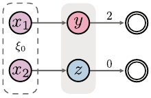
Figure 9.1

A Markov decision process in which aliasing due to function approximation may result

in the wrong value function estimates even at the unaliased states x

and x

to map two-dimensional points to a desired action, usually by predicting the

return obtained following this action.

While there are similarities between the use of probability distribution rep-

resentations (parameterizing the output of a return function) and function

approximation (parameterizing its input), the latter requires a diﬀerent algorith-

mic treatment. When function approximation is required, it is usually because

it is infeasible to exhaustively enumerate the state space and apply dynamic

programming methods. One solution is to rely on samples (of the state space,

transitions, trajectories, etc.), but this results in additional complexities in the

algorithm’s design. Combining incremental algorithms with function approxi-

mation may result in instability or even divergence; in the distributional setting,

the analysis of these algorithms is complicated by two levels of approximation

(one for probability distributions and one across states). With proper care, how-

ever, function approximation provides an eﬀective way of dealing with large

reinforcement learning problems.

9.1 Function Approximation and Aliasing

By necessity, when parameters are shared across states, a single parameter usu-

ally aﬀects the predictions (value or distribution) at multiple states. In this case,

we say that the states are aliased. State aliasing has surprising consequences in

the context of reinforcement learning, including the unwanted propagation of

errors and potential instability in the learning process.

Example 9.1.

Consider the Markov decision process in Figure 9.1, with four

nonterminal states

, x

, y

, and

, a single action, a deterministic reward

function, an initial state distribution

, and no discounting. Consider an

68.

Domains such as Mountain Car – which have a single initial state and a deterministic transition

function – can be solved without function approximation: for example, by means of a search

algorithm. However, function approximation allows us to learn a control policy that can in theory

be applied to any given state and has a low run-time cost.

Draft version.

Linear Function Approximation 263

approximation based on three parameters w

, w

, and w

, such that

V(x

) = w

V(x

) = w

V(y) =

V(z) = w

Because the rewards from

and

are diﬀerent, no choice of

can yield

V = V

. As such, any particular choice of w

trades oﬀ approximation error at

and

. When a reinforcement learning algorithm is combined with function

approximation, this trade-oﬀ is made (implicitly or explicitly) based on the

algorithm’s characteristics and the parameters of the learning process. For

example, the best approximation obtained by the incremental Monte Carlo

algorithm (Section 3.2) correctly learns the value of x

and x

V(x

) = 2 ,

V(x

) = 0 ,

but learns a parameter

that depends on the frequency at which states

and

are visited. This is because

is updated toward 2 whenever the estimate

(

) is updated and toward 0 whenever

(

) is updated. In our example, the

frequency at which this occurs is directly implied by the initial state distribution

, and we have

= 2 ×P

= y) + 0 ×P

= z)

= 2ξ

) . (9.1)

When the approximation is learned using a bootstrapping procedure, aliasing

can also result in incorrect estimates at states that are not themselves aliased.

The solution found by temporal-diﬀerence learning,

, is as per Equation 9.1,

but the algorithm also learns the incorrect value at x

and x

V(x

) =

V(x

) = 0 + γ ×

V(z)

= 2ξ

) .

Thus, errors due to function approximation can compound in unexpected ways;

we will study this phenomenon in greater detail in Section 9.3. 4

In a linear value function approximation, the value estimate at a state

given by a weighted combination of features of

. This is in opposition to a

tabular representation, where value estimates are stored in a table with one

entry per state.

As we will see, linear approximation is simple to implement

and relatively easy to analyze.

Deﬁnition 9.2.

Let

n ∈N

. A state representation is a mapping

X→R

A linear value function approximation

∈R

is parameterized by a weight

69.

Technically, a tabular representation can also be expressed using the trivial collection of indicator

features. In practice, the two are used in distinct problem settings.

Draft version.

264 Chapter 9

vector w ∈R

and maps states to their expected return estimates according to

(x) = φ(x)

w .

A feature

(

)

∈R

= 1

, . . . , n

is an individual element of

(

). We call the

vectors φ

∈R

basis functions. 4

As its name implies, a linear value function approximation is linear in the

weight vector w. That is, for any w

, w

∈R

, α, β ∈R, we have

αw

+βw

= αV

+ βV

In addition, the gradient of V

(x) with respect to w is given by

∇

(x) = φ(x) .

As we will see, these properties aﬀect the learning dynamics of algorithms that

use linear value function approximation.

We extend linear value function approximation to state-action values in the

usual way. For a state representation φ : X×A→R

, we deﬁne

(x, a) = φ(x, a)

w .

A practical alternative is to use a distinct set of weights for each action and a

common representation

(

) across actions. In this case, we use a collection of

weight vectors (w

: a ∈A), with w

∈R

, and write

(x, a) = φ(x)

Remark 9.1 discusses the relationship between these two methods.

9.2 Optimal Linear Value Function Approximations

In this chapter, we will assume that there is a ﬁnite (but very large) number

of states. In this case, the state representation

X→R

can expressed as a

feature matrix Φ

∈R

X×n

whose rows are the vectors

(

x ∈X

. This yields the

approximation

= Φw .

The state representation determines a space of value function approximations

that are constructed from linear combinations of features. Expressed in terms of

the feature matrix, this space is

= {Φw : w ∈R

We ﬁrst consider the problem of ﬁnding the best linear approximation to a value

function

. Because

is a

-dimensional linear subspace of the space of

value functions

, there are necessarily some value functions that cannot be

represented with a given state representation (unless

). We measure the

Draft version.

Linear Function Approximation 265

discrepancy between a value function

and an approximation

= Φ

ξ-weighted L

norm, for ξ ∈P(X):

−V

ξ,2



x∈X

ξ(x)



(x) −V

(x)





The weighting

reﬂects the relative importance given to diﬀerent states. For

example, we may weigh states according to the frequency at which they are

visited, or we may put greater importance on initial states. Provided that

(

)

for all x ∈X, the norm k·k

ξ,2

induces the ξ-weighted L

metric on R

ξ,2

(V, V

) = kV −V

ξ,2

The best linear approximation under this metric is the solution to the

minimization problem

min

w∈R

−V

ξ,2

. (9.2)

One advantage of measuring approximation error in a weighted

norm, rather

than the

∞

norm used in the analyses of previous chapters, is that a solution

∗

to Equation 9.2 can be easily determined by solving a least-squares system.

Proposition 9.3.

Suppose that the columns of the feature matrix Φ are

linearly independent and

(

)

0 for all

x ∈X

. Then, Equation 9.2 has a

unique solution w

∗

given by

∗

= (Φ

ΞΦ)

−1

ΞV

, (9.3)

where Ξ ∈R

X×X

is a diagonal matrix with entries (ξ(x) : x ∈X). 4

Proof. By a standard calculus argument, any optimum w must satisfy

∇

x∈X

ξ(x)



(x) −φ(x)



= 0

=⇒

x∈X

ξ(x)



(x) −φ(x)



φ(x) = 0 .

Written in matrix form, this is

Ξ(Φw −V

) = 0

=⇒ Φ

ΞΦw = Φ

ΞV

70.

Technically,

k·k

ξ,2

is only a proper norm if

is strictly positive for all

; otherwise, it is

a semi-norm. Under the same condition,

ξ,2

is proper metric; otherwise, it is a pseudo-metric.

Assuming that ξ(x) > 0 for all x addresses uniqueness issues and simpliﬁes the analysis.

Draft version.

266 Chapter 9

Because Φ has rank

, then so does Φ

ΞΦ: for any

u ∈R

with

u ,

0, we have

Φu = v , 0 and so

ΞΦu = v

Ξv

x∈X

ξ(x)v(x)

> 0 ,

(

)

0 and

(

)

≥

0 for all

x ∈X

, and

x∈X

(

)

0. Hence, Φ

ΞΦ is

invertible and the only solution w

∗

to the above satisﬁes Equation 9.3.

9.3 A Projected Bellman Operator for Linear Value Function

Approximation

Dynamic programming ﬁnds an approximation to the value function

successively computing the iterates

k+1

= T

As we saw in preceding chapters, dynamic programming makes it easy to derive

incremental algorithms for learning the value from samples and also allows us to

ﬁnd an approximation to the optimal value function

∗

. Often, it is the de facto

approach for ﬁnding an approximation of the return-distribution function. It is

also particularly useful when using function approximation, where it enables

algorithms that learn by extrapolating to unseen states.

When dynamic programming is combined with function approximation, we

obtain a range of methods called approximate dynamic programming. In the case

of linear value function approximation, the iterates (

)

k≥0

are given by linear

combinations of features, which allows us to apply dynamic programming to

problems with larger state spaces than can be described in memory. In general,

however, the space of approximations

is not closed under the Bellman

operator, in the sense that

V ∈F

6=⇒ T

V ∈F

Similar to the notion of a distributional projection introduced in Chapter 5, we

address the issue by projecting, for

V ∈R

, the value function

back onto

. Let us deﬁne the projection operator Π

φ,ξ

: R

→R

(Π

φ,ξ

V)(x) = φ(x)

∗

such that w

∗

∈arg min

w∈R

kV −V

ξ,2

This operator returns the approximation

∗

= Φ

∗

that is closest to

V ∈R

in the

-weighted

norm. As established by Proposition 9.3, when

is fully

supported on

and the basis functions (

)

i=1

are linearly independent, then this

Draft version.

Linear Function Approximation 267

projection is unique.

By repeatedly applying the projected Bellman operator

φ,ξ

from an initial condition V

∈F

, we obtain the iterates

k+1

= Π

φ,ξ

. (9.4)

Unlike the approach taken in Chapter 5, however, it is usually impractical

to implement Equation 9.4 as is, as there are too many states to enumerate.

A simple solution is to rely on a sampling procedure that approximates the

operator itself. For example, one may sample a batch of

states and ﬁnd the

best linear ﬁt to

at these states. In the next section, we will study the

related approach of using an incremental algorithm to learn the linear value

function approximation from sample transitions. Understanding the behavior

of the exact projected operator Π

φ,ξ

informs us about the behavior of these

approximations, as it describes in some sense the ideal behavior that one expects

from both of these approaches.

Also diﬀerent from the setting of Chapter 5 is the presence of aliasing across

states. As a consequence of this aliasing, we have limited freedom in the choice

of projection if we wish to guarantee the convergence of the iterates of Equation

9.4. To obtain such a guarantee, in general, we need to impose a condition on

the distribution

that deﬁnes the projection Π

φ,ξ

. We will demonstrate that

the projected Bellman operator is a contraction mapping with modulus

with

respect to the

-weighted

norm, for a speciﬁc choice of

. Historically, this

approach predates the analysis of distributional dynamic programming and is in

fact a key inspiration for our analysis of distributional reinforcement learning

algorithms as approximating projected Bellman operators (see bibliographical

remarks).

To begin, let us introduce the convention that the Lipschitz constant of an

operator with respect to a norm (such as

∞

) follows Deﬁnition 5.20, applied to

the metric associated with the norm. In the case of

∞

, this metric deﬁnes the

distance between u, u

∈R

ku −u

∞

Now recall that the Bellman operator

is a contraction mapping in

∞

norm,

with modulus

. One reason this holds is because the transition matrix

satisﬁes

∞

≤kuk

∞

, for all u ∈R

;

71.

If only the ﬁrst of those two conditions hold, then there may be multiple optimal weight vectors.

However, they all result in the same value function, and the projection remains unique.

Draft version.

268 Chapter 9

we made use of this fact in the proof of Proposition 4.4. This is equivalent to

requiring that the Lipschitz constant of P

satisfy

∞

≤1 .

Unfortunately, the Lipschitz constant of Π

φ,ξ

in the

∞

norm may be greater

than 1, precluding a direct analysis in that norm (see Exercise 9.5). We instead

prove that the Lipschitz constant of

in the

-weighted

norm satisﬁes the

same condition when

is taken to be a steady-state distribution under policy

Deﬁnition 9.4.

Consider a Markov decision process and let

be a policy

deﬁning the probability distribution

over the random transition (

X, A, R, X

We say that ξ ∈P(X) is a steady-state distribution for π if for all x

∈X,

ξ(x

) =

x∈X

ξ(x)P

= x

| X = x) . 4

Assumption 9.5.

There is a unique steady-state distribution

, and it satisﬁes

(x) > 0 for all x ∈X. 4

Qualitatively, Assumption 9.5 ensures that approximation error at any state

is reﬂected in the norm

k·k

; contrast with the setting in which

is nonzero

only at a handful of states. Uniqueness is not strictly necessary but simpliﬁes the

exposition. There are a number of practical scenarios in which the assumption

does not hold, most importantly when there is a terminal state. We discuss how

to address such a situation in Remark 9.2.

Lemma 9.6.

Let

X→P

(

) be a policy and let

be a steady-state distri-

bution for this policy. The transition matrix is a nonexpansion with respect to

the ξ

-weighted L

metric. That is,

= 1 . 4

Proof.

A simple algebraic argument shows that if

U ∈R

is such that

(

) = 1

for all x, then

U = U .

This shows that kP

≥1. Now for an arbitrary U ∈R

, write

x∈X

(x)



U)(x)



x∈X

(x)



∈X

| x)U(x

)



(a)

≤

x∈X

(x)

∈X

| x)



U(x

)



Draft version.

Linear Function Approximation 269

∈X



U(x

)



x∈X

(x)P

| x)

(b)

∈X

)



U(x

)



= kUk

where (a) follows by Jensen’s inequality and (b) by Deﬁnition 9.4. Since

= sup

U∈R

kUk

≤1 ,

this concludes the proof.

Lemma 9.7.

For any

ξ ∈P

(

) with

(

)

0, the projection operator Π

φ,ξ

is a

nonexpansion in the ξ-weighted L

metric, in the sense that

kΠ

φ,ξ

ξ,2

= 1 . 4

The proof constitutes Exercise 9.4.

Theorem 9.8.

Let

be a policy and suppose that Assumption 9.5 holds;

let

be the corresponding steady-state distribution. The projected Bellman

operator Π

φ,ξ

is a contraction with respect to the

-weighted

norm

with modulus γ, in the sense that for any V, V

∈R

kΠ

φ,ξ

V −Π

φ,ξ

≤γkV −V

As a consequence, this operator has a unique ﬁxed point

= Π

φ,ξ

, (9.5)

which satisﬁes

−V

≤

1 −γ

kΠ

φ,ξ

−V

. (9.6)

In addition, for an initial value function V

∈R

, the sequence of iterates

k+1

= Π

φ,ξ

(9.7)

converges to this ﬁxed point. 4

Proof.

The contraction result and consequent convergence of the iterates in

Equation 9.7 to a unique ﬁxed point follow from Lemmas 9.6 and 9.7, which,

combined with Lemma 5.21, allow us to deduce that

kΠ

φ,ξ

≤γ .

Draft version.

270 Chapter 9

Because Assumption 9.5 guarantees that

k·k

induces a proper metric, we

may then apply Banach’s ﬁxed-point theorem. For the error bound of Equation

9.6, we use Pythagoras’s theorem to write

−V

= k

−Π

φ,ξ

+ kΠ

φ,ξ

−V

= kΠ

φ,ξ

−Π

φ,ξ

+ kΠ

φ,ξ

−V

≤γ

−V

+ kΠ

φ,ξ

−V

since

φ,ξ

≤γ

. The result follows by rearranging terms and taking the

square root of both sides.

Theorem 9.8 implies that the iterates (

)

k≥0

are guaranteed to converge

when the projection is performed in

-weighted

norm. Of course, this does

not imply that a projection in a diﬀerent norm may not result in a convergent

algorithm (see Exercise 9.8), but divergence is a practical concern (we return to

this point in the next section). A sound alternative to imposing a condition on

the distribution

is to instead impose a condition on the feature matrix Φ; this

is explored in Exercise 9.10.

When the feature matrix Φ forms a basis of

(i.e., it has rank

), it is

always possible to ﬁnd a weight vector w

∗

for which

Φw

∗

= T

V ,

for any given V ∈R

. As a consequence, for any ξ ∈P (X) we have

φ,ξ

= T

and Theorem 9.8 reduces to the analysis of the (unprojected) Bellman operator

given in Section 4.2. On the other hand, when

n < N

, the ﬁxed point of Equation

9.5 is in general diﬀerent from the minimum-error solution Π

φ,ξ

and is

called the temporal-diﬀerence learning ﬁxed point. Similar to the diﬀusion

eﬀect studied in Section 5.8, successive applications of the projected Bellman

operator result in compounding approximation errors. The nature of this ﬁxed

point is by now well studied in the literature (see bibliographical remarks).

9.4 Semi-Gradient Temporal-Diﬀerence Learning

We now consider the design of a sample-based, incremental algorithm for

learning the linear approximation of a value function

. In the context of

domains with large state spaces, algorithms that learn from samples have an

advantage over dynamic programming approaches: whereas the latter require

some form of enumeration and hence have a computational cost that depends

on the size of

, the computational cost of the former instead depends on the

Draft version.

Linear Function Approximation 271

size of the function approximation (in the linear case, on the number of features

n).

To begin, let us consider learning a linear value function approximation using

an incremental Monte Carlo algorithm. We are presented with a sequence of

state-return pairs (

, g

)

k≥0

, with the assumption that the source states

are

realizations of independent draws from the distribution

and that each

is a

corresponding independent realization of the random return

(

). As before,

we are interested in the optimal weight vector w

∗

for the problem

min

w∈R

−V

ξ,2

, V

(x) = φ(x)

w . (9.8)

Of note, the optimal approximation V

∗

is also the solution to the problem

min

w∈R

E[kG

−V

ξ,2

] . (9.9)

Consequently, a simple approach for ﬁnding

∗

is to perform stochastic gradient

descent with a loss function that reﬂects Equation 9.9. For

x ∈X

and

z ∈R

, let

us deﬁne the sample loss

L(w) =



z −φ(x)



whose gradient with respect to w is

∇

L(w) = −2



z −φ(x)



φ(x) .

Stochastic gradient descent updates the weight vector

by following the (nega-

tive) gradient of the sample loss constructed from each sample. Instantiating

the sample loss with x = x

and z = g

, this results in the update rule

w ←w + α

−φ(x

)



φ(x

) , (9.10)

where

∈

1) is a time-varying step size that also subsumes the constant

from the loss. Under appropriate conditions, this update rule ﬁnds the optimal

weight vector

∗

(see, e.g., Bottou 1998). Exercise 9.9 asks you to verify that

the optimal weight vector w

∗

is a ﬁxed point of the expected update.

Let us now consider the problem of learning the value function from a

sequence of sample transitions (

, a

, r

, x

)

k≥0

, again assumed to be indepen-

dent realizations from the appropriate distributions. Given a weight vector

the temporal-diﬀerence learning target for linear value function approximation

+ γV

) = r

+ γφ(x

)

w .

We use this target in lieu of

in Equation 9.10 to obtain the semi-gradient

temporal-diﬀerence learning update rule

w ←w + α



+ γφ(x

)

w −φ(x

)



| {z }

TD error

φ(x

) , (9.11)

Draft version.

272 Chapter 9

in which the temporal-diﬀerence (TD) error appears, now with value function

estimates constructed from linear approximation. By substituting the Monte

Carlo target

for the temporal-diﬀerence target, the intent is to learn an

approximation to

by a bootstrapping process, as in the tabular setting. The

term “semi-gradient” reﬂects the fact that the update rule does not actually

follow the gradient of the sample loss



+ γφ(x

)

w −φ(x

)



which contains additional terms related to φ(x

) (see bibliographical remarks).

We can understand the relationship between semi-gradient temporal-

diﬀerence learning and the projected Bellman operator Π

φ,ξ

by way of an

update rule deﬁned in terms of a second set of weights

˜w

, the target weights.

This update rule is

w ←w + α

+ γφ(x

)

˜w −φ(x

)



φ(x

) . (9.12)

When

˜w

, this is Equation 9.11. However, if

˜w

is a separate weight vector,

this is the update rule of stochastic gradient descent on the sample loss



+ γφ(x

)

˜w −φ(x

)



Consequently, this update rule ﬁnds a weight vector

∗

that approximately

minimizes

˜w

−V

ξ,2

and Equation 9.12 describes an incremental algorithm for computing a single

step of the projected Bellman operator applied to V

˜w

; its solution w

∗

satisﬁes

Φw

∗

= Π

φ,ξ

˜w

This argument suggests that semi-gradient temporal-diﬀerence learning tracks

the behavior of the projected Bellman operator. In particular, at the ﬁxed point

= Φ

ˆw

of this operator, semi-gradient TD learning (applied to realizations

from the sample transition model (

X, A, R, X

), with

X ∼ξ

) leaves the weight

vector unchanged, in expectation.



R + γφ(X

)

ˆw −φ(X)

ˆw



φ(X)



= 0 .

In semi-gradient temporal-diﬀerence learning, however, the sample target

γφ

(

)

depends on

and is used to update

itself. This establishes

a feedback loop that, combined with function approximation, can result in

divergence – even when the projected Bellman operator is well behaved. The

following example illustrates this phenomenon.

Draft version.

Linear Function Approximation 273

0 20 40 60 80 100

Iteration

Approximation error (log)

(a) (b)

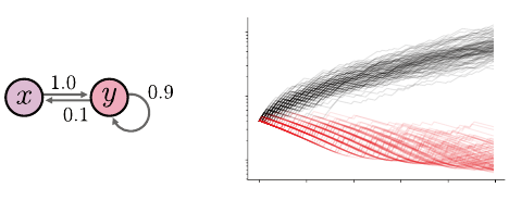
Figure 9.2

(a)

A Markov decision process for which semi-gradient temporal-diﬀerence learning can

diverge.

(b)

Approximation error (measured in unweighted

norm) over the course of

100 runs of the algorithm with

= 0

01 and the same initial condition

= (1

0) but

diﬀerent draws of the sample transitions. Black and red lines indicate runs with

(

) =

and

/11, respectively.

Example 9.9

(Baird’s counterexample (Baird 1995))

Consider the Markov

decision process depicted in Figure 9.2a and the state representation

φ(x) = (1, 3, 2) φ(y) = (4, 3, 3).

Since the reward is zero everywhere, the value function for this MDP is

= 0.

However, if X

∼ξ with ξ(x) = ξ(y) = 1/2, the semi-gradient update

k+1

= w

+ α(0 + γφ(X

)

−φ(X

)

)φ(X

)

diverges unless

= 0. Figure 9.2b depicts the eﬀect of this divergence on the

approximation error: on average, the distance to the ﬁxed point

−

ξ,2

grows exponentially with each update. Also shown is the approximation error

over time if we take ξ to be the steady-state distribution

ξ(x) =

/11 ξ(y) =

/11,

in which case the approximation error becomes close to zero as

k →∞

. This

demonstrates the impact of the relative update frequency of diﬀerent states on

the behavior of the algorithm.

On the other hand, note that the basis functions implied by

span

and

thus

φ,ξ

V = T

for any

V ∈R

. Hence, the iterates

k+1

= Π

φ,ξ

in this case converge to

0 for any initial

∈R

. This illustrates that requiring the convergence that

the sequence of iterates derived from the projected Bellman operator is not

suﬃcient to guarantee the convergence of the semi-gradient iterates. 4

Draft version.

274 Chapter 9

Example 9.9 illustrates how reinforcement learning with function approx-

imation is a more delicate task than in the tabular setting. If states are

updated proportionally to their steady-state distribution, however, a convergence

guarantee becomes possible (see bibliographical remarks).

9.5 Semi-Gradient Algorithms for Distributional Reinforcement

Learning

With the right modeling tools, function approximation can also be used to

tractably represent the return functions of large problems. One diﬀerence with

the expected-value setting is that it is typically more challenging to construct

an approximation that is linear in the true sense of the word. With linear

value function approximations, adding weight vectors is equivalent to adding

approximations:

(x) = V

(x) + V

(x) .

In the distributional setting, the same cannot apply because probability dis-

tributions do not form a vector space. This means that we cannot expect a

return-distribution function representation to satisfy

(x)

= η

(x) + η

(x) ; (9.13)

the right-hand side is not a probability distribution (it is, however, a signed

distribution: more on this in Section 9.6). An alternative is to take a slightly

broader view and consider distributions whose parameters depend linearly on

. There are now two sources of approximation: one due to the ﬁnite parameter-

ization of probability distributions in

, another because those parameters are

themselves aliased. This is an expressive framework, albeit one under which

the analysis of algorithms is signiﬁcantly more complex.

Linear QTD.

Let us ﬁrst derive a linear approximation of quantile temporal-

diﬀerence learning. Linear QTD represents the locations of quantile distri-

butions using linear combinations of features. If we write

w ∈R

m×n

for the

matrix whose columns are

, . . . , w

∈R

, then the linear QTD return function

estimate takes the form

(x) =

i=1

φ(x)

One can verify that

(

) is not a linear combination of features, even though

its parameters are. We construct the linear QTD update rule by following the

negative gradient of the quantile loss (Equation 6.12), taken with respect to the

parameters w

, . . . , w

. We ﬁrst rewrite this loss in terms of a function ρ

(∆) = |

{∆ < 0}

−τ|×|∆|

Draft version.

Linear Function Approximation 275

so that for a sample

z ∈R

and estimate

θ ∈R

, the loss of Equation 6.12 can be

expressed as

{z < θ}

−τ|×|z −θ|= ρ

(z −θ) .

We instantiate the quantile loss with

(

)

and

2i−1

to obtain the

loss

(w) = ρ

(z −φ(x)

) . (9.14)

By the chain rule, the gradient of this loss with respect to w

∇

(z −φ(x)

) = −(τ

− {z < φ(x)

})φ(x) . (9.15)

As in our derivation of QTD, from a sample transition (

x, a, r, x

), we construct

m sample targets:

= r + γφ(x

)

, j = 1, . . . , m .

By instantiating the gradient expression in Equation 9.15 with

and taking

the average over the m sample targets, we obtain the update rule

←w

−α

j=1

∇



−φ(x)



which is more explicitly

←w

+ α

j=1



− {g

< φ(x)

}



| {z }

quantile TD error

φ(x). (9.16)

Note that, by plugging

into the expression for the gradient (Equation 9.15),

we obtain a semi-gradient update rule. That is, analogous to the value-based

case, Equation 9.16 is not equivalent to the gradient update

←w

−α

j=1

∇



r + γφ(x

)

−φ(x)



because in general

∇



r + γφ(x

)

−φ(x)





− {g

< φ(x)

}



φ(x) .

Linear CTD.

To derive a linear approximation of categorical temporal-

diﬀerence learning, we represent the probabilities of categorical distributions

using linear combinations of features. Speciﬁcally, we apply the softmax func-

tion to transform the parameters (

(

)

i=1

into a probability distribution. We

write

(x; w) =

φ(x)

j=1

φ(x)

. (9.17)

Draft version.

276 Chapter 9

Recall that the probabilities



(

;

))

i=1

correspond to

locations (

)

i=1

. The

softmax transformation guarantees that the expression

(x) =

i=1

(x; w)δ

describes a bona ﬁde probability distribution. We thus construct the sample

target ¯η(x):

¯η(x) = Π

r,γ

)

) = Π

i=1

; w)δ

r+γθ

i=1

¯p

where

¯p

denotes the probability assigned to the location

by the sample target

¯η

(

). Expressed in terms of the CTD coeﬃcients (Equation 6.10), the probability

¯p

j=1

i, j

(r)p

; w) .

As with quantile regression, we adjust the weights

by means of a gradient

descent procedure. Here, we use the cross-entropy loss between

(

) and

¯η(x):

L(w) = −

i=1

¯p

log p

(x; w). (9.18)

Combined with the softmax function, Equation 9.18 becomes

L(w) = −

i=1

¯p



φ(x)

−log

j=1

φ(x)



With some algebra and again invoking the chain rule, we obtain that the gradient

with respect to the weights w

∇

L(w) = −



¯p

− p

(x; w)



φ(x) .

By adjusting the weights in the opposite direction of this gradient, this results

in the update rule

←w

+ α



¯p

− p

(x; w)



| {z }

CTD error

φ(x). (9.19)

72.

The choice of cross-entropy loss is justiﬁed because it is the matching loss for the softmax

function, and their combination results in a convex objective (Auer et al. 1995; see also Bishop

2006, Section 4.3.6).

Draft version.

Linear Function Approximation 277

While interesting in their own right, linear CTD and QTD are particularly

important in that they can be straightforwardly adapted to learn return-

distribution functions with nonlinear function approximation schemes such

as deep neural networks; we return to this point in Chapter 10. For now, it is

worth noting that the update rules of linear TD, linear QTD, and linear CTD

can all be expressed as

←w

+ αε

φ(x) ,

where

is an error term. One interesting diﬀerence is that for both linear

CTD and linear QTD,

lies in the interval [

−

1], while for linear TD, it

is unbounded. This gives evidence that we should expect diﬀerent learning

dynamics from these algorithms. In addition, combining linear TD or linear

QTD to a tabular state representation recovers the corresponding incremen-

tal algorithms from Chapter 6. For linear CTD, the update corresponds to a

tabular representation of the softmax parameters rather than the probabilities

themselves, and the correspondence is not as straightforward.

Analyzing linear QTD and CTD is complicated by the fact that the return

functions themselves are not linear in

, . . . , w

. One solution is to relax the

requirement that the approximation

(

) be a probability distribution; as we

will see in the next section, in this case the distributional approximation behaves

much like the value function approximation, and a theoretical guarantee can be

obtained.

9.6 An Algorithm Based on Signed Distributions*

So far, we made sure that the outputs of our distributional algorithms were valid

probability distributions (or could be as interpreted as such: for example, when

working with statistical functionals). This was done explicitly when using the

softmax parameterization in deﬁning linear CTD and implicitly in the mixture

update rule of CTD in Chapter 3. In this section, we consider an algorithm that

is similar to linear CTD but omits the softmax function. As a consequence of

this change, this modiﬁed algorithm’s outputs are signed distributions, which

we brieﬂy encountered in Chapter 6 in the course of analyzing categorical

temporal-diﬀerence learning.

Compared to linear CTD, this approach has the advantage of being both

closer to the tabular algorithm (it ﬁnds a best ﬁt in



distance, like tabular

CTD) and closer to linear value function approximation (making it amenable

to analysis). Although the learned predictions lack some aspects of probability

distributions – such as well-deﬁned quantiles – the learned signed distributions

can be used to estimate expectations of functions, including expected values.

Draft version.

278 Chapter 9

To begin, let us deﬁne a (ﬁnite) signed distribution

as a weighted sum of

two probability distributions:

ν = λ

+ λ

, λ

∈R , ν

, ν

∈P(R) . (9.20)

We write

(

) for the space of ﬁnite signed distributions. For

ν ∈M

(

)

decomposed as in Equation 9.20, we deﬁne its cumulative distribution function

and the expectation of a function f : R →R as

(z) = λ

(z) + λ

(z), z ∈R

Z∼ν

[ f (Z)] = λ

Z∼ν

[ f (Z)] + λ

Z∼ν

[ f (Z)] . (9.21)

Exercise 9.14 asks you to verify that these deﬁnitions are independent of the

decomposition of

into a sum of probability distributions. The total mass of

is given by

κ(ν) = λ

+ λ

We make these deﬁnitions explicit because signed distributions are not proba-

bility distributions; in particular, we cannot draw samples from

. In that sense,

the notation

Z ∼ν

in the deﬁnition of expectation is technically incorrect, but

we use it here for convenience.

Deﬁnition 9.10.

The signed

-categorical representation parameterizes the

mass of m particles at ﬁxed locations (θ

)

i=1

S,m

i=1

: p

∈R for i = 1, . . . , m,

i=1

= 1

. 4

Compared to the usual

-categorical representation, its signed analogue

adds a degree of freedom: it allows the mass of its particles to be negative and

of magnitude greater than 1 (we reserve “probability” for values strictly in

1]). However, in our deﬁnition, we still require that signed

-categorical

distributions have unit total mass; as we will see, this avoids a number of

technical diﬃculties. Exercise 9.15 asks you to verify that ν ∈F

S,m

is a signed

distribution in the sense of Equation 9.20.

Recall from Section 5.6 that the categorical projection Π

(

)

→F

C,m

deﬁned in terms of the triangular and half-triangular kernels

R →

1],

, . . . , m

. We use Equation 9.21 to extend this projection to signed distributions,

written Π

(

)

→F

S,m

. Given

ν ∈M

(

), the masses of Π

i=1

are

given by

= E

Z∼ν





−1

(Z −θ

)



where as before,

−1

i+1

−θ

(

i < m

), and we write

Z∼ν

in the sense of Equation

9.21. We also extend the notation to signed return-distribution functions in the

Draft version.

Linear Function Approximation 279

usual way. Observe that if

is a probability distribution, then Π

matches our

earlier deﬁnition. The distributional Bellman operator, too, can be extended

to signed distributions. Let

η ∈M

(

)

be a signed return function. We deﬁne

: M (R)

→M (R)

η)(x) = E

[(b

R,γ

)

η(X

) |X = x] .

This is the same equation as before, except that now the operator constructs

convex combinations of signed distributions.

Deﬁnition 9.11.

Given a state representation

X→R

and evenly spaced

particle locations

, …, θ

, a signed linear return function approximation

∈F

S,m

is parameterized by a weight matrix

w ∈R

n×m

and maps states to

signed return function estimates according to

(x) =

i=1

(x; w)δ

, p

(x; w) = φ(x)



1 −

j=1

φ(x)



, (9.22)

where

is the

th column of

. We denote the space of signed return functions

that can be represented in this form by F

φ,S,m

. 4

Equation 9.22 can be understood as approximating the mass of each particle

linearly and then adding mass to all particles uniformly to normalize the signed

distribution to have unit total mass. It deﬁnes a subset of signed

-categorical

distributions that are constructed from linear combinations of features. Because

of the normalization, and unlike the space of linear value function approxima-

tions constructed from

φ,S,m

is not a linear subspace of

(

). However,

for each x ∈X, the mapping

w 7→η

(x)

is said to be aﬃne, a property that is suﬃcient to permit theoretical analysis

(see Remark 9.3).

Using a linearly parameterized representation of the form given in Equa-

tion 9.22, we seek to build a distributional dynamic programming algorithm

based on the signed categorical representation. The complication now is that the

distributional Bellman operator takes the return function approximation away

from our linear parameterization in two separate ways: ﬁrst, the distributions

themselves may move away from the categorical representation, and second, the

distributions may no longer be representable by a linear combination of features.

We address these issues with a doubly projected distributional operator:

φ,ξ,

where the outer projection ﬁnds the best approximation to Π

in F

φ,S,m

. By

analogy with the value-based setting, we deﬁne “best approximation” in terms

Draft version.

280 Chapter 9

of a ξ-weighted Cramér distance, denoted 

ξ,2



(ν, ν

) =

(z) −F

(z))

dz ,



ξ,2

(η, η

) =

x∈X

ξ(x)



η(x), η

(x)



φ,ξ,

η = arg min

∈F

φ,S,m



ξ,2

(η, η

) .

Because we are now dealing with signed distributions, the Cramér distance



(

ν, ν

) is inﬁnite if the two input signed distributions

ν, ν

do not have the same

total mass. This justiﬁes our restriction to signed distributions with unit total

mass in deﬁning both the signed

-categorical representation and the linear

approximation. The following lemma shows that the distributional Bellman

operator preserves this property (see Exercise 9.16).

Lemma 9.12.

Suppose that

η ∈M

(

)

is a signed return-distribution function.

Then,



η)(x)



∈X

= x

| X = x)κ



η(x

)



In particular, if all distributions of

have unit total mass – that is,

(

)) = 1

for all x – then



η)(x)



= 1 . 4

While it is possible to derive algorithms that are not restricted to outputting

signed distributions with unit total mass, one must then deal with added com-

plexity due to the distributional Bellman operator moving total mass from state

to state.

We next derive a semi-gradient update rule based on the doubly projected

Bellman operator. Following the unbiased estimation method for designing

incremental algorithms (Section 6.2), we construct the signed target

˜η(x) = Π

r,γ

)

) .

Compared to the sample target of Equation 6.9, here

is a signed return

function in F

S,m

The semi-gradient update rule adjusts the weight vectors

to minimize the



distance between Π

˜η

(

) and the predicted distribution

(

). It does so by

taking a step in direction of the negative gradient of the squared 

distance

←w

−α∇



(η

(x), Π

˜η(x)) .

73. In this expression, ˜η(x) is used as a target estimate and treated as constant with regards to w.

Draft version.

Linear Function Approximation 281

We obtain an implementable version of this update rule by expressing distri-

butions in

S,m

in terms of

-dimensional vectors of masses. For a signed

categorical distribution

ν =

i=1

let us denote by

p ∈R

the vector (

, …, p

); similarly, denote by

the

vector of masses for a signed distribution

. Because the cumulative functions

of signed categorical distributions with unit total mass are constant on the

intervals [θ

, θ

i+1

] and equal outside of the [θ

, θ

] interval, we can write



(ν, ν

) =



(z) −F

(z)



= ς

m−1

i=1



(θ

) −F

(θ

)



= ς

kCp −C p

, (9.23)

where

k·k

is the usual Euclidean norm and

C ∈R

m×m

is the lower-triangular

matrix

C =







1 0 ··· 0 0

1 1 ··· 0 0

1 1 ··· 1 0

1 1 ··· 1 1







Letting

(

) and

˜p

(

) denote the vector of masses for the signed approximation

(

) and the signed target Π

˜η

(

), respectively, we rewrite the above in terms

of matrix-vector operations (Exercise 9.17 asks you to derive the gradient of



with respect to w

←w

+ ας

( ˜p(x) − p(x))

C ˜e

φ(x) , (9.24)

where ˜e

∈R

is a vector whose entries are

˜e

i j

{i = j}

−

By precomputing the vectors

C ˜e

, this update rule can be applied in

(

mn) operations per sample transition.

9.7 Convergence of the Signed Algorithm*

We now turn our attention to establishing a contraction result for the doubly

projected Bellman operator, by analogy with Theorem 9.8. We write



(R) = {λ

+ λ

: λ

, λ

∈R, λ

+ λ

= 1, ν

, ν

∈P



(R)},

Draft version.

282 Chapter 9

for ﬁnite signed distributions with unit total mass and ﬁnite Cramér distance

from one another. In particular, note that F

S,m

⊆M



(R).

Theorem 9.13.

Suppose Assumption 4.29(1) holds and that Assump-

tion 9.5 holds with unique stationary distribution

. Then the pro-

jected operator Π

φ,ξ

,



(

)

→M



(

)

is a contraction with

respect to the metric 

, with contraction modulus γ

. 4

This result is established by analyzing separately each of the three operators

that composed together constitute the doubly projected operator Π

φ,ξ

,

Lemma 9.14.

Under the assumptions of Theorem 9.13,



(

)

→



(R) is a γ

-contraction with respect to 

. 4

Lemma 9.15.

The categorical projection operator Π



(

)

→F

S,m

is a

nonexpansion with respect to 

. 4

Lemma 9.16.

Under the assumptions of Theorem 9.13, the function approxima-

tion projection operator Π

φ,ξ

,

S,m

→F

S,m

is a nonexpansion with respect

to 

. 4

The proof of Lemma 9.14 essentially combines the reasoning of Proposi-

tion 4.20 and Lemma 9.6 and so is left as Exercise 9.18. Similarly, the proof of

Lemma 9.15 follows according to exactly the same calculations as in the proof

of Lemma 5.23, and so it is left as Exercise 9.19. The central observation is

that the corresponding arguments made for the Cramér distance in Chapter 5

under the assumption of probability distributions do not actually make use of

the monotonicity of the cumulative distribution functions and so extend to the

signed distributions under consideration here.

Proof of Lemma 9.16.

Let

η, η

∈F

S,m

and write

(

) for the vector of

masses of η(x) and η

(x), respectively. From Equation 9.23, we have



(η, η

) =

x∈X

(x)

(η(x), η

(x))

x∈X

(x)ς

kCp(x) −C p

(x)k

= ς

kp − p

Ξ⊗C

where Ξ

⊗C

is a positive semi-deﬁnite matrix in

(X×m)×(X×m)

, with Ξ =

diag

(

)

∈R

X×X

, and

p, p

∈R

X×m

are the vectorized probabilities associated

with

η, η

. Therefore, Π

φ,ξ

,

can be interpreted as a Euclidean projection under

Draft version.

Linear Function Approximation 283

the norm

k·k

Ξ⊗C

and hence is a nonexpansion with respect to the corre-

sponding norm; the result follows as this norm precisely induces the metric



Proof of Theorem 9.13.

We use similar logic to that of Lemma 5.21 to com-

bine the individual contraction results established above, taking care that the

operators to be composed have several diﬀerent domains between them. Let

η, η

∈M



(R)

. Then note that



(Π

φ,ξ

,

η, Π

φ,ξ

,

)

(a)

≤

(Π

η, Π

)

(b)

≤

η, T

)

(c)

≤γ



(η, η

) ,

as required. Here, (a) follows from Lemma 9.16, since Π

η,

∈

S,m

. (b) follows from Lemma 9.15 and the straightforward corollary that



(Π

η,

)

≤

(

η, η

) for

η, η

∈M



(

). Finally, (c) follows from

Lemma 9.14.

The categorical projection is a useful computational device as it allows Π

φ,ξ,

to be implemented strictly in terms of signed

-categorical representations,

and we rely on it in our analysis. Mathematically, however, it is not strictly

necessary as it is implied by the projection onto the

φ,S,m

; this is demonstrated

by the following Pythagorean lemma.

Lemma 9.17.

For any signed

-categorical distribution

ν ∈F

S,m

(for which

ν = Π

ν) and any signed distribution ν

∈M



(R),



(ν, ν

) = 

(ν, Π

) + 

(Π

, ν

) . (9.25)

Consequently, for any η ∈M



(R),

φ,ξ,

η = Π

φ,ξ,

η . 4

Equation 9.25 is obtained by a similar derivation to the one given in Remark

5.4, which proves the identity when

and

are the usual

-categorical

distributions.

Just as in the case studied in Chapter 5 without function approximation, it

is now possible to establish a guarantee on the quality of the ﬁxed point of the

operator Π

φ,ξ

,

Draft version.

284 Chapter 9

Proposition 9.18.

Suppose that the conditions of Theorem 9.13 hold, and

let

ˆη

be the resulting ﬁxed point of the projected operator Π

φ,ξ

,

We have the following guarantee on the quality of

ˆη

compared with the

(

2,ξ

, F

φ,S,m

)-optimal approximation of η

: namely, Π

φ,ξ

,



(η

, ˆη

) ≤



(η

, Π

φ,ξ

,

)

1 −γ

. 4

Proof. We calculate directly:



(η

, ˆη

)

(a)

= 

(η

, Π

φ,ξ

,

) + 

(Π

φ,ξ

,

, Π

φ,ξ

,

ˆη

)

(b)

= 

(η

, Π

φ,ξ

,

) + 

(Π

φ,ξ

,

, Π

φ,ξ

,

ˆη

)

(c)

≤ 

(η

, Π

φ,ξ

,

) + γ

(η

, ˆη

)

=⇒ 

(η

, ˆη

) ≤

1 −γ



(η

, Π

φ,ξ

,

) ,

where (a) follows from the Pythagorean identity in Lemma 9.17 and a similar

identity concerning Π

φ,ξ

,

, (b) follows since

is ﬁxed by

and

ˆη

is ﬁxed

by Π

φ,ξ

,

, and (c) follows from

-contractivity of Π

φ,ξ

,



2,ξ

This result provides a quantitative guarantee on how much the approximation

error compounds when

ˆη

is computed by approximate dynamic programming.

Of note, here there are two sources of error: one due to the use of a ﬁnite

number

of distributional parameters and another due to the use of function

approximation.

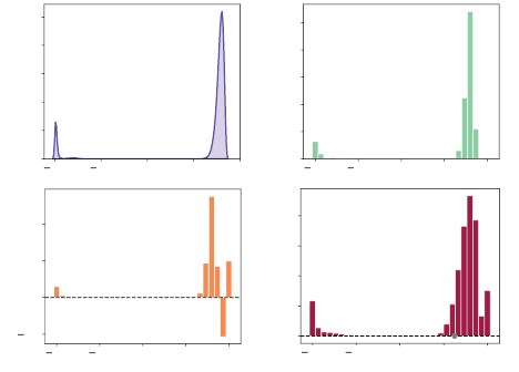
Example 9.19.

Consider linearly approximating the return-distribution func-

tion of the safe policy in the Cliﬀs domain (Example 2.9). If we use a

three-dimensional state representation

(

) = [1

, x

, r

] where

, x

are the

row and column indices of a given state, then we observe aliasing in the

approximated return distribution (Figure 9.3). In addition, the use of a signed

distribution representation results in negative mass being assigned to some

locations in the optimal approximation. This is by design; given the limited

capacity of the approximation, the algorithms ﬁnd a solution that mitigates

errors at some locations by introducing negative mass at other locations. As

usual, the use of a bootstrapping procedure introduces diﬀusion error, here quite

signiﬁcant due to the low-dimensional state representation. 4

Draft version.

Linear Function Approximation 285

1.0 0.5 0.0 0.5 1.0

Return

Density

1.0 0.5 0.0 0.5 1.0

Return

0.2

0.0

0.2

0.4

Mass

1.0 0.5 0.0 0.5 1.0

Return

0.00

0.05

0.10

0.15

0.20

Mass

1.0 0.5 0.0 0.5 1.0

Return

0.0

0.1

0.2

0.3

0.4

0.5

Probability

(a) (b)

Figure 9.3

Signed linear approximations of the return distribution of the initial state in Example 2.9.

(a–b)

Ground-truth return-distribution function and categorical Monte Carlo approxima-

tion, for reference. (

) Best approximation from

φ,S,m

based on the state representation

(

) = [1

, x

, r

] where

, x

are the row and column indices of a given state, with (0

denoting the top-left corner. (d) Fixed point of the signed categorical algorithm.

9.8 Technical Remarks

Remark 9.1.

For ﬁnite action spaces, we can easily convert a state represen-

tation

(

) to a state-action representation

(

x, a

) by repeating a basic feature

matrix Φ

∈R

X×n

. Let

be the number of actions. We build a block-diagonal

feature matrix Φ

X,A

∈R

(X×A)×(nN

)

that contains N

copies of Φ:

X,A







Φ 0 ··· 0

0 Φ ··· 0

0 0 ··· Φ







The weight vector w is also extended to be of dimension nN

, so that

(x, a) =



X,A



(x, a)

as before. This is equivalent to but somewhat more verbose than the use of

per-action weight vectors. 4

Remark 9.2.

Assumption 9.5 enabled us to demonstrate that the projected

Bellman operator Π

φ,ξ

has a unique ﬁxed point, by invoking Banach’s ﬁxed

point theorem. The ﬁrst part of the assumption, on the uniqueness of

, is

relatively mild and is only used to simplify the exposition. However, if there

Draft version.

286 Chapter 9

is a state

for which

(

) = 0, then

k·k

does not deﬁne a proper metric on

and Banach’s theorem cannot be used. In this case, there might be multiple

ﬁxed points (see Exercise 9.7).

In addition, if we allow

to assign zero probability to some states, the

norm

k·k

may not be a very interesting measure of accuracy. One common

situation where the issue arises is when there is a terminal state

∅

that is

reached with probability 1, in which case

lim

t→∞

= x

∅

) = 1 .

It is easy to see that in this case,

puts all of its probability mass on

∅

, so

that Theorem 9.8 becomes vacuous: the norm

k·k

only measures the error at

the terminal state. A more interesting distribution to consider is the distribution

of states resulting from immediately resetting to an initial state when

∅

reached. In particular, this corresponds to the distribution used in many practical

applications. Let

be the initial state distribution; without loss of generality,

let us assume that ξ

∅

) = 0. Deﬁne the substochastic transition operator

X,∅

| x, a) =

(

0 if x

= x

∅

| x, a) otherwise.

In addition, deﬁne a transition operator that replaces transitions to the terminal

state by transition to one of the initial states, according to the initial distribution

X,ξ

| x, a) = P

X,∅

| x, a) +

, x

∅

}

∅

| x, a)ξ

) .

One can show that the Bellman operator T

∅

(deﬁned from P

X,∅

) satisﬁes

∅

V = T

for any

V ∈R

for which

(

∅

) = 0 and that the steady-state distribution

∅

induced by P

X,ξ

and a policy π is such that

there exists t ∈N, P

= x) > 0 =⇒ ξ

∅

(x) > 0 .

Let P

∅

be the transition matrix corresponding to P

X,∅

| x, a) and the policy

π. Exercise 9.21 asks you to prove that

∅

≤1 ,

from which a modiﬁed version of Theorem 9.8 can be obtained. 4

Remark 9.3.

Let

and

be vector spaces. A mapping

M → M

is said

to be aﬃne if, for any U, U

∈ M and α ∈[0, 1],

O(αU + (1 −α)U

) = αOU + (1 −α)OU

Draft version.

Linear Function Approximation 287

When

is a signed linear return function approximation parameterized by

the map

w 7→η

(x)

is aﬃne for each

x ∈X

, as we now show. It is this property that allows us to

express the



distance between

ν, ν

∈F

S,m

in terms of a diﬀerence of vectors

of probabilities (Equation 9.23), needed in the proof of Lemma 9.16.

Let

w, w

∈R

n×m

be the parameters of signed return functions of the form of

Equation 9.22. For these, write

(

) for the vector of masses determined by

(x) = w

φ(x) +



1 −e

φ(x)



where e is the m-dimensional vector of ones. We then have

i=1

φ(x)

= e

φ(x) ,

and similarly for w

. Hence,

αw+(1−α)w

(x) = (αw + (1 −α)w

)

φ(x) −

(αw + (1 −α)w

)

φ(x)

= αp

(x) + (1 −α)p

(x) .

We conclude that w 7→η

(x) is indeed aﬃne in w. 4

9.9 Bibliographical Remarks

9.1–9.2.

Linear value function approximation as described in this book is in

eﬀect a special case of linear regression where the inputs are taken from a

ﬁnite set (

(

))

x∈X

and noiseless labels; see Strang (1993), Bishop (2006),

and Murphy (2012) for a discussion on linear regression. Early in the history

of reinforcement learning research, function approximation was provided by

connectionist systems (Barto et al. 1983; Barto et al. 1995) and used to deal

with inﬁnite state spaces (Boyan and Moore 1995; Sutton 1996). An earlier-still

form of linear function approximation and temporal-diﬀerence learning was

used by Samuel (1959) to train a strong player for the game of checkers.

9.3.

Bertsekas and Tsitsiklis (1996, Chapter 6) studies linear value function

approximation and its combination with various reinforcement learning meth-

ods, including TD learning (see also Bertsekas 2011, 2012). Tsitsiklis and Van

Roy (1997) establish the contractive nature of the projected Bellman operator

φ,ξ

under the steady-state distribution (Theorem 9.8 in this book). The

temporal-diﬀerence ﬁxed point can be determined directly by solving a least-

squares problem, yielding the least-squares TD algorithm (LSTD; Bradtke and

Barto 1996), which is extended to the control setting by least-squares policy

Draft version.

288 Chapter 9

iteration (LSPI; Lagoudakis and Parr 2003). In the control setting, the method is

also called ﬁtted Q-iteration (Gordon 1995; Ernst et al. 2005; Riedmiller 2005).

Bertsekas (1995) gives an early demonstration that the TD ﬁxed point is in

general diﬀerent from (and has greater error than) the best approximation to

, measured in

-weighted

norm. However, it is possible to interpret the

temporal-diﬀerence ﬁxed point as the solution to an oblique projection problem

that minimizes errors between consecutive states (Harmon and Baird 1996;

Scherrer 2010).

9.4.

Barnard (1993) provides a proof that temporal-diﬀerence learning is not

a true gradient-descent method, justifying the term semi-gradient (Sutton and

Barto 2018). The situation in which

diﬀers from the steady-state (or sampling)

distribution of the induced Markov chain is called oﬀ-policy learning; Example

9.9 is a simpliﬁed version of the original counterexample due to Baird (1995).

Baird argued for the direct minimization of the Bellman residual by gradient

descent as a replacement to temporal-diﬀerence learning, but this method suﬀers

from other issues and can produce undesirable solutions even in mild scenarios

(Sutton et al. 2008a). The GTD line of work (Sutton et al. 2009; Maei 2011)

is a direct attempt at handling the issue by using a pair of approximations (see

Qu et al. 2019 for applications of this idea in a distributional context); more

recent work directly considers a corrected version of the Bellman residual (Dai

et al. 2018; Chen and Jiang 2019). The convergence of temporal-diﬀerence

learning with linear function approximation was proven under fairly general

conditions by Tsitsiklis and Van Roy (1997), using the ODE method from

stochastic approximation theory (Benveniste et al. 2012; Kushner and Yin 2003;

Ljung 1977).

Parr et al. (2007), Parr et al. (2008) and Sutton et al. (2008b) provide a domain-

dependent analysis of linear value function approximation, which is extended

by Ghosh and Bellemare (2020) to establish the existence of representations

that are stable under a greater array of conditions (Exercises 9.10 and 9.11).

Kolter (2011) studies the space of temporal-diﬀerence ﬁxed point as a function

of the distribution ξ.

9.5.

Linear CTD and QTD were implicitly introduced by Bellemare et

al. (2017a) and Dabney et al. (2018b), respectively, in the design of deep

reinforcement learning agents (see Chapter 10). Their presentation as given

here is new.

9.6–9.7.

The algorithm based on signed distributions is new to this book. It

improves on an algorithm proposed by Bellemare et al. (2019b) in that it adjusts

the total mass of return distributions to always be 1. Lyle et al. (2019) give

evidence that the original algorithm generally underperforms the categorical

Draft version.

Linear Function Approximation 289

algorithm. They further establish that, in the risk-neutral control setting, distri-

butional algorithms cannot do better than value-based algorithms when using

linear approximation. The reader interested in the theory of signed measures is

referred to Doob (1994).

9.10 Exercises

Exercise 9.1.

Use the update rules of Equation 9.10 and 9.11 to prove the

results from Example 9.1. 4

Exercise 9.2.

Prove that for a linear value function approximation

= Φ

we have, for any w, w

∈R

and α, β ∈R,

αw+βw

= αV

+ βV

, ∇

(x) = φ(x). 4

Exercise 9.3. In the statement of Proposition 9.3, we required that

(i) the columns of the feature matrix Φ be linearly independent;

(ii) ξ(x) > 0 for all x ∈X.

Explain how the result is aﬀected when either of these requirements is omitted.

Exercise 9.4.

Prove Lemma 9.7. Hint. Apply Pythagoras’s theorem to a well-

chosen inner product. 4

Exercise 9.5.

The purpose of this exercise is to empirically study the con-

tractive and expansive properties of the projection in

norm. Consider an

integer-valued state space

x ∈X

{

, . . . ,

}

with two-dimensional state rep-

resentation

(

) = (1

, x

), and write Π

for the

projection of a vector

v ∈R

onto the linear subspace deﬁned by φ. That is,

v = Φ(Φ

Φ)

−1

where Φ is the feature matrix.

With this representation, we can represent the vector

(

) = 0 exactly, and

hence Π

u = u. Now consider the vector u

deﬁned by

(x) = log x.

With a numerical experiment, show that

kΠ

−Π

≤ku

−uk

but kΠ

−Π

∞

> ku

−uk

∞

. 4

Exercise 9.6.

Provide an example Markov decision process and state represen-

tation that result in the left- and right-hand sides of Equation 9.6 being equal.

Hint. A diagram might prove useful. 4

Draft version.

290 Chapter 9

Exercise 9.7.

Following Remark 9.2, suppose that the steady-state distribution

is such that

(

) = 0 for some state

. Discuss the implications on the analysis

performed in this chapter, in particular on the set of solutions to Equation 9.8

and the behavior of semi-gradient temporal-diﬀerence learning when source

states are drawn from this distribution. 4

Exercise 9.8.

Let

be some initial distribution and

a policy. Deﬁne the

discounted state-visitation distribution

ξ(x

) = (1 −γ)ξ

) + γ

x∈X

= x

| X = x)

ξ(x), for all x

∈X.

Following the line of reasoning leading to Lemma 9.6, show that the projected

Bellman operator Π

φ,ξ

is a γ

contraction in the

ξ-weighted L

metric:

ξ,2

≤γ

. 4

Exercise 9.9.

Let

ξ ∈P

(

). Suppose that the feature matrix Φ

∈R

X×n

has

linearly independent columns and

(

)

0 for all

x ∈X

. Show that the unique

optimal weight vector w

∗

that is a solution to Equation 9.2 satisﬁes



(X) −φ(X)

∗



φ(X)

= 0, X ∼ξ. 4

Exercise 9.10

(*)

This exercise studies the divergence of semi-gradient

temporal-diﬀerence learning from a dynamical systems perspective. Recall

that Ξ ∈R

X×X

is the diagonal matrix whose entries are ξ(x).

(i)

Show that in expectation and in matrix form, Equation 9.11 produces the

sequence of weight vectors (w

)

k≥0

given by

k+1

= w

+ α



+ γP

Φw

−Φw

(ii) Assume that α

= α > 0. Express the above as an update of the form

k+1

= Aw

+ b, (9.26)

where A ∈R

n×n

and b ∈R

(iii)

Suppose that the matrix

= Φ

Ξ(

γP

−I

)Φ has eigenvalues that are all

real. Show that if one of these is positive, then

has at least one eigenvalue

greater than 1.

(iv)

Use the preceding result to conclude that under those conditions, there

exists a w

such that kw

→∞.

(v)

Suppose now that all of the matrix

’s eigenvalues are real and nonpositive.

Show that in this case, there exists an α ∈(0, 1) such that taking α

= α, the

sequence (Φw

)

k≥0

converges to the temporal-diﬀerence ﬁxed point. 4

Exercise 9.11 (*). Suppose that the state representation is such that

(i) the matrix P

Φ ∈R

X×n

has columns that lie in the column span of Φ, and

Draft version.

Linear Function Approximation 291

(ii)

the matrix has columns that are orthogonal with regards to the

-weighted

inner product. That is,

ΞΦ = I.

Show that in this case, the eigenvalues of the matrix

Ξ(γP

−I)Φ

are all nonpositive, for any choice of

ξ ∈P

(

). Based on the previous exercise,

conclude on the dynamical properties of semi-gradient temporal-diﬀerence

learning with this representation. 4

Exercise 9.12.

Using your favorite numerical computation software, implement

the Markov decision process from Baird’s counterexample (Example 9.9) and

the semi-gradient update

k+1

= w

+ α



γφ(x

−φ(x



φ(x

) ,

for the state representation of the example and a small, constant value of

Here, it is assumed that

has distribution

and

is drawn from the transition

kernel depicted in Figure 9.2.

(i)

Vary

(

) from 0 to 1, and plot the norm of the value function estimate,

ξ,2

, as a function of k.

(ii)

Now replace

(

)

(

)

˜w

, where

˜w

k−k mod L

for some integer

L ≥

1. That is,

˜w

is kept ﬁxed for

iterations. Plot the evolution of

ξ,2

for diﬀerent values of L. What do you observe? 4

Exercise 9.13.

Repeat Exercise 3.3, replacing the uniform grid encoding the

state with a representation φ deﬁned by

φ(x) =



1, sin(x

), cos(x

), …, sin(x

), cos(x

)



where (

, x

) denote the Cart–Pole state variables. Implement linear CTD and

QTD and use these with the state representation

to learn a return-distribution

function approximation for the uniform and forward-leaning policies. Visualize

the learned approximations at selected states, including the initial state, and com-

pare them to ground-truth return distributions estimated by the nonparametric

Monte Carlo algorithm (Remark 3.1). 4

Exercise 9.14.

Recall that given a ﬁnite signed distribution

expressed as a

sum of probability distributions

(with

, λ

∈R

, ν

∈P

(

)),

we deﬁned expectations under

in terms of sums of expectations under

and

. Verify that this deﬁnition is not dependent on the choice of decomposi-

tion of

into a sum of probability distributions. That is, suppose that there

also exist

, λ

∈R

and

, ν

∈P

(

) with

. Show that for any

Draft version.

292 Chapter 9

(measurable) function f : R →R with

Z∼ν

[|f (Z)|] < ∞, E

Z∼ν

[|f (Z)|] < ∞, E

Z∼ν

[|f (Z)|] < ∞, E

Z∼ν

[|f (Z)|] < ∞,

we have

Z∼ν

[ f (Z)] + λ

X∼ν

[ f (Z)] = λ

Z∼ν

[ f (Z)] + λ

Z∼ν

[ f (Z)] . 4

Exercise 9.15.

Show that any

-categorical signed distribution

ν ∈F

S,m

can

be written as the weighted sum of two

-categorical (probability) distributions

, ν

∈F

C,m

. 4

Exercise 9.16.

Suppose that we consider a return function

η ∈M

(

)

deﬁned

over signed distributions (not necessarily with unit total mass). Show that



η)(x)



∈X

= x | X = x)κ(η(x

)) .

Conclude that if η ∈F

S,m

, then



η)(x)



= 1 . 4

Exercise 9.17.

Consider two signed

-categorical distributions

ν, ν

∈F

S,m

Denote their respective vectors of masses by

p, p

∈R

. Prove the correctness

of Equation 9.24. That is, show that

∇



(ν, ν

) = −2ς

− p)

C ˜e

φ(x) . 4

Exercise 9.18. Prove Lemma 9.14. 4

Exercise 9.19. Prove Lemma 9.15. 4

Exercise 9.20. Prove Lemma 9.17. 4

Exercise 9.21. Following the discussion in Remark 9.2, show that

∅

≤1 . 4

Draft version.