8
Statistical Functionals
The development of distributional reinforcement learning in previous chapters
has focused on approximating the full return function with parameterized fami-
lies of distributions. In our analysis, we quantified the accuracy of an algorithm’s
estimate according to its distance from the true return-distribution function,
measured using a suitable probability metric.
Rather than try to approximate the full distribution of the return, we may
instead select specific properties of this distribution and directly estimate these
properties. Implicitly, this is the approach taken when estimating the expected
return. Other common properties of interest include quantiles of the distribu-
tions, high-probability tail bounds, and the risk-sensitive objectives described in
Chapter 7. In this chapter, we introduce the language of statistical functionals
to describe such properties.
In some cases, the statistical functional approach allows us to obtain accurate
estimates of quantities of interest, in a more straightforward manner. As a
concrete example, there is a low-cost dynamic programming procedure to
determine the variance of the return distribution.
61
By contrast, categorical and
quantile dynamic programming usually under- or overestimate this variance.
This chapter develops the framework of statistical functional dynamic pro-
gramming as a general method for approximately determining the values of
statistical functionals. As we demonstrate in Section 8.4, it is in fact possible
to interpret both categorical and quantile dynamic programming as operating
over statistical functionals. We will see that while some characteristics of the
return (including its variance) can be accurately estimated by an iterative proce-
dure, in general, some care must be taken when estimating arbitrary statistical
functionals.
61.
In fact, the return variance can be determined to machine precision by solving a linear system
of equations, similar to what was done in Section 5.1 for the value function.
Draft version. 233
234 Chapter 8
8.1 Statistical Functionals
A functional maps functions to real values. By extension, a statistical functional
maps probability distributions to the reals. In this book, we view statistical
functionals as measuring a particular property or characteristic of a probability
distribution. For example, the mapping
ν 7→P
Z∼ν
Z ≥0
, ν ∈P(R)
is a statistical functional that measures how much probability mass its argument
ν
puts on the nonnegative reals. Statistical functionals express quantifiable
properties of probability distributions such as their mean and variance. The
following formalizes this point.
Definition 8.1.
A statistical functional
ψ
is a mapping from a subset of
probability distributions P
ψ
(R) ⊆P(R) to the reals, written
ψ : P
ψ
(R) →R .
We call the particular scalar
ψ
(
ν
) associated with a probability distribution
ν
a
functional value and the set P
ψ
(R) the domain of the functional. 4
Example 8.2.
The mean functional maps probability distributions to their
expected values. As before, let
P
1
(R) = {ν ∈P(R) : E
Z∼ν
|Z|
< ∞}
be the set of distributions with finite first moment. For
ν ∈P
1
(
R
), the mean
functional is
µ
1
(ν) = E
Z∼ν
[Z] .
The restriction to
P
1
(
R
) is necessary to exclude from the definition distributions
without a well-defined mean. 4
The purpose of this chapter is to study how functional values of the return
distribution can be approximated using dynamic programming procedures and
incremental algorithms. In general, we will be interested in a collection of
such functionals that exhibit desirable properties: for example, because they
can be jointly determined by dynamic programming or because they provide
complementary information about the return function. We call such a collection
a distribution sketch.
Definition 8.3.
A distribution sketch (or simply sketch)
ψ
:
P
ψ
(
R
)
→R
m
is a
vector-valued function specified by a tuple (
ψ
1
, …, ψ
m
) of statistical functionals.
Its domain is
P
ψ
(R) =
m
\
i=1
P
ψ
i
(R) ,
Draft version.
Statistical Functionals 235
and it is defined as
ψ(ν) = (ψ
1
(ν), …, ψ
m
(ν)), ν ∈P
ψ
(R) .
Its image is
I
ψ
=
ψ(ν) : ν ∈P
ψ
(R)
⊆R
m
.
We also extend this notation to return-distribution functions:
ψ(η) =
ψ(η(x)) : x ∈X), η ∈P
ψ
(R)
X
. 4
Example 8.4.
The quantile functionals are a family of statistical function-
als indexed by
τ ∈
(0
,
1) and defined over
P
(
R
). The
τ
-quantile functional is
defined in terms of the inverse cumulative distribution function of its argument
(Definition 4.12):
ψ
q
τ
(ν) = F
−1
ν
(τ) .
A finite collection of quantile functionals (say, for
τ
1
, . . . , τ
m
∈
(0
,
1)) constitutes
a sketch. 4
Example 8.5.
To prove the convergence of categorical temporal-difference
learning (Section 6.10), we introduced the isometry I: F
C,m
→R
I
defined as
I(ν) =
F
ν
(θ
i
) : i ∈{1, . . . , m}
, (8.1)
where (
θ
i
)
m
i=1
is the set of locations for the categorical representation. This
isometry is also a sketch in the sense of Definition 8.3. If we extend its domain
to be
P
(
R
), Equation 8.1 still defines a valid sketch but it is no longer an
isometry: it is not possible to recover the distribution
ν
from its functional
values I(ν). 4
8.2 Moments
Moments are an especially important class of statistical functionals. For an
integer p ∈N
+
, the pth moment of a distribution ν ∈P
p
(R) is given by
µ
p
(ν) = E
Z∼ν
Z
p
.
In particular, the first moment of
ν
is its mean, while the variance of
ν
is the
difference between its second moment and squared mean:
µ
2
(ν) −
µ
1
(ν)
2
. (8.2)
Moments are ubiquitous in mathematics. They form a natural way of capturing
important aspects of a probability distribution, and the infinite sequence of
moments
µ
p
(
ν
)
∞
p=1
uniquely characterizes many probability distributions of
interest; see Remark 8.3.
Draft version.
236 Chapter 8
Our goal in this section is to describe a dynamic programming approach to
determining the moments of the return distribution. Fix a policy
π
, and consider
a state
x ∈X
and action
a ∈A
. The
p
th moment of the return distribution
η
π
(
x, a
)
is given by
E
π
h
G
π
(x, a)
p
i
,
where as before,
G
π
(
x, a
) is an instantiation of
η
π
(
x, a
). Although we can also
study dynamic programming approaches to learning the
p
th moment of state-
indexed return distributions,
E
π
h
G
π
(x)
p
i
,
this is complicated by a potential conditional dependency between the reward
R
and next state
X
0
due to the action
A
. One solution is to assume independence
of
R
and
X
0
, as we did in Section 5.4. Here, however, to avoid making this
assumption, we work with functions indexed by state-action pairs.
To begin, let us fix m ∈N
+
. The m-moment function M
π
is
M
π
(x, a, i) = E
π
[(G
π
(x, a))
i
] = µ
i
η
π
(x, a)
, for i = 1, . . . , m . (8.3)
As with value functions, we view
M
π
as the function (or vector) in
R
X×A×m
describing the collection of the first
m
moments of the random return. In
particular,
M
π
(
·, ·,
1) is the usual state-action value function. As elsewhere in
the book, to ensure that the expectation in Equation 8.3 is well defined, we
assume that all reward distributions have finite
p
th moments, for
p
= 1
, . . . , m
.
In fact, it is sufficient to assume that this holds for
p
=
m
(Assumption 4.29(
m
)).
As with the standard Bellman equation, from the state-action random-
variable Bellman equation
G
π
(x, a) = R + γG
π
(X
0
, A
0
), X = x, A = a
we can derive Bellman equations for the moments of the return distribution. To
do so, we raise both sides to the
i
th power and take expectations with respect
to both the random return variables
G
π
and the random transition (
X
=
x, A
=
a, R, X
0
, A
0
):
E
π
[(G
π
(x, a))
i
] = E
π
[(R + γG
π
(X
0
, A
0
))
i
| X = x, A = a] .
From the binomial expansion of the term inside the expectation, we obtain
E
π
[(G
π
(x, a))
i
] = E
π
i
X
j=0
γ
i−j
i
j
!
R
j
G
π
(X
0
, A
0
)
i−j
X = x, A = a
.
Draft version.

Statistical Functionals 237
Since
R
and
G
π
(
X
0
, A
0
) are independent given
X
and
A
, we can rewrite the above
as
M
π
(x, a, i) =
i
X
j=0
γ
i−j
i
j
!
E
π
[R
j
| X = x, A = a] E
π
M
π
(X
0
, A
0
, i − j) | X = x, A = a
,
where by convention we take
M
π
(
x
0
, a
0
,
0) = 1 for all
x
0
∈X
and
a
0
∈A
. This is a
recursive characterization of the
i
th moment of a return distribution, analogous
to the familiar Bellman equation for the mean. The recursion is cast into the
familiar framework of operators with the following definition.
Definition 8.6.
Let
m ∈N
+
. The
m
-moment Bellman operator
T
π
(m)
:
R
X×A×m
→
R
X×A×m
is given by
(T
π
(m)
M)(x, a, i) = (8.4)
i
X
j=0
γ
i−j
i
j
!
E
π
[R
j
| X = x, A = a] E
π
M(X
0
, A
0
, i − j) | X = x, A = a
. 4
The collection of moments (
M
π
(
x, a, i
) : (
x, a
)
∈X×A, i
= 1
, …, m
) is a fixed
point of the operator
T
π
(m)
. In general, the
m
-moment Bellman operator is not a
contraction mapping with respect to the
L
∞
metric (except, of course, for
m
= 1;
see Exercise 8.1). However, with a more nuanced analysis, we can still show
that T
π
(m)
has a unique fixed point to which the iterates
M
k+1
= T
π
(m)
M
k
(8.5)
converge.
Proposition 8.7.
Let
m ∈N
+
. Under Assumption 4.29(
m
),
M
π
is the
unique fixed point of
T
π
(m)
. In addition, for any initial condition
M
0
∈
R
X×A×m
, the iterates of Equation 8.5 converge to M
π
. 4
Proof.
We begin by constructing a suitable notion of distance between
m
-
moment functions R
X×A×m
. For M ∈R
X×A×m
, let
kMk
∞,i
= sup
(x,a)∈X×A
|M(x, a, i)|, for i = 1, . . . , m
kMk
∞,<i
= sup
j=1,…,i−1
kMk
∞, j
, for i = 2, . . . , m .
Each of
k·k
∞,i
(for
i
= 1
, …, m
) and
k·k
∞,<i
(for
i
= 2
, …, m
) is a semi-norm; they
fulfill the requirements of a norm, except that neither
kMk
∞,i
= 0 nor
kMk
∞,<i
= 0
implies that M = 0. From these semi-norms, we construct the pseudo-metrics
(M, M
0
) 7→kM − M
0
k
∞,i
,
Draft version.
238 Chapter 8
noting that it is possible for the distance between
M
and
M
0
to be zero even
when M is different from M
0
.
The structure of the proof is to argue that
T
π
(m)
is a contraction with modulus
γ
with respect to
k·k
∞,1
and then to show inductively that it satisfies an inequality
of the form
kT
π
(m)
M −T
π
(m)
M
0
k
∞,i
≤C
i
kM −M
0
k
∞,<i
+ γ
i
kM −M
0
k
∞,i
, (8.6)
for each
i
= 2
, …, m
, and some constant
C
i
that depends on
P
R
. Chaining these
results together then leads to the convergence statement, and uniqueness follows
as an immediate corollary.
To see that
T
π
(m)
is a contraction with respect to
k·k
∞,1
, let
M ∈R
X×A×m
, and
write
M
(i)
= (
M
(
x, a, i
) : (
x, a
)
∈X×A
) for the function in
R
X×A
corresponding
to the
i
th moment function estimates given by
M
. By inspecting Equation 8.4
with i = 1, it follows that
T
π
(m)
M
(1)
= T
π
M
(1)
,
where
T
π
is the usual Bellman operator. Furthermore,
kMk
∞,1
=
kM
(1)
k
∞
, and
so the statement that
T
π
(m)
is a contraction with respect to the pseudo-metric
implied by
k·k
∞,1
is equivalent to the contractivity of
T
π
on
R
X×A
with the
respect to the L
∞
norm, which was shown in Proposition 4.4.
To see that
T
π
(m)
satisfies the bound of Equation 8.6 for
i >
1, let
L ∈R
be such
that
E[R
i
| X = x, A = a]
≤L, for all x, a ∈X×A and i = 1, …, m.
Observe that
(T
π
(m)
M)(x, a, i) −(T
π
(m)
M
0
)(x, a, i)
=
i−1
X
j=0
γ
i−j
i
j
!
E
π
R
j
|X = x, A = a
×
X
x
0
∈X
a
0
∈A
P
X
(x
0
| x, a)π(a
0
| x
0
)(M −M
0
)(x
0
, a
0
, i − j)
≤
i−1
X
j=1
γ
i−j
i
j
!
E
π
R
j
|X = x, A = a
×kM − M
0
k
∞,<i
+ γ
i
kM −M
0
k
∞,i
≤L
i−1
X
j=1
γ
i−j
i
j
!
kM −M
0
k
∞,<i
+ γ
i
kM −M
0
k
∞,i
≤(2
i
−2)LkM − M
0
k
∞,<i
+ γ
i
kM −M
0
k
∞,i
.
Draft version.

Statistical Functionals 239
Taking C
i
= (2
i
−2)L, we have
kT
π
(m)
M −T
π
(m)
M
0
k
∞,i
≤C
i
kM −M
0
k
∞,<i
+ γ
i
kM −M
0
k
∞,i
, for i = 2, . . . , m.
To chain these results together, first observe that
kM
k
− M
π
k
∞,1
→0.
We next argue inductively that if, for a given
i < m
, (
M
k
)
k≥0
converges to
M
π
in
the pseudo-metric induced by k·k
∞,<i
, then also
kM
k
− M
π
k
∞,i
→0, and hence
kM
k
− M
π
k
∞,<(i+1)
→0.
Let
y
k
=
kM
k
− M
π
k
∞,<i
and
z
k
=
kM
k
− M
π
k
∞,i
. Then the generalized contraction
result states that
z
k+1
≤C
i
y
k
+
γ
i
z
k
. Taking the limit superior on both sides yields
lim sup
k→∞
z
k
≤lim sup
k→∞
C
i
y
k
+ γ
i
z
k
= γ
i
lim sup
k→∞
z
k
,
where we have used the result
y
k
→
0. From this, we deduce
lim sup
k→∞
z
k
≤
0,
but since (
z
k
)
k≥0
is a nonnegative sequence, we therefore have
z
k
→
0. This
completes the inductive step, and we therefore obtain
kM
k
− M
π
k
∞,i
→
0, as
required.
In essence, Proposition 8.7 establishes that the
m
-moment Bellman operator
behaves in a similar fashion to the usual Bellman operator, in the sense that its
iterates converge to the fixed point
M
π
. From here, we may follow the deriva-
tions of Chapter 5 to construct a dynamic programming algorithm for learning
these moments
62
or those of Chapter 6 to construct the corresponding incre-
mental algorithm (Section 8.8). Although the proof above does not demonstrate
the contractive nature of the moment Bellman operator, for
m
= 2, this can be
achieved using a different norm and analysis technique (Exercise 8.4).
8.3 Bellman Closedness
In preceding chapters, our approach to distributional reinforcement learning
considered approximations of the return distributions that could be tractably
manipulated by algorithms. The
m
-moment Bellman operator, on the other
hand, is not directly applied to probability distributions – compared to say,
a
m
-categorical distribution, there is no immediate procedure for drawing a
sample from a collection of
m
moments. Compared to the categorical and
62.
When the reward distributions take on a finite number of values, in particular, the expectations
of Definition 8.6 can be implemented as sums.
Draft version.
240 Chapter 8
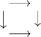
η η
0
s s
0
T
π
ψ
ψ
T
π
ψ
Figure 8.1
A sketch is Bellman closed if there is an operator
T
π
ψ
such that in the diagram above, the
composite functions ψ ◦T
π
and T
π
ψ
◦ψ coincide.
quantile projected operators, however, the
m
-moment operator yields an error-
free dynamic programming procedure – with sufficiently many iterations and
under some finiteness assumptions, we can determine the moments of the
return function to any degree of accuracy. The concept of Bellman closedness
formalizes this idea.
Definition 8.8.
A sketch
ψ
= (
ψ
1
, …, ψ
m
) is Bellman closed if, whenever its
domain P
ψ
(R)
X
is closed under the distributional Bellman operator:
η ∈P
ψ
(R)
X
=⇒ T
π
η ∈P
ψ
(R)
X
,
there is an operator T
π
ψ
: I
X
ψ
→I
X
ψ
such that
ψ
T
π
η
= T
π
ψ
ψ
η
for all η ∈P
ψ
(R)
X
.
The operator T
π
ψ
is said to be the Bellman operator for the sketch ψ. 4
As was demonstrated in the preceding section, the collection of the
m
first
moments
µ
1
, . . . , µ
m
is a Bellman-closed sketch. Its associated operator is the
m-moment operator T
π
(m)
.
When a sketch
ψ
is Bellman closed, the operator
T
π
ψ
mirrors the application
of the distributional Bellman operator to the return-distribution function
η
; see
Figure 8.1. The concept of Bellman closedness is related to that of a diffusion-
free projection (Chapter 5), and we will in fact establish an equivalence between
the two in Section 8.4. In addition, Bellman-closed sketches are particularly
interesting from a computational perspective because they support an exact
dynamic programming procedure, as the following establishes.
Draft version.

Statistical Functionals 241
Proposition 8.9.
Let
ψ
= (
ψ
1
, …, ψ
m
) be a Bellman-closed sketch and sup-
pose that
P
ψ
(
R
)
X
is closed under
T
π
. Then for any initial condition
η
0
∈P
ψ
(R)
X
, and sequences (η
k
)
k≥0
, (s
k
)
k≥0
defined by
η
k+1
= T
π
η
k
, s
0
= ψ(η
0
) , s
k+1
= T
π
ψ
s
k
,
we have, for k ≥0,
s
k
= ψ(η
k
) .
In addition, the functional values
s
π
=
ψ
(
η
π
) of the return-distribution
function are a fixed point of the operator T
π
ψ
. 4
Proof.
Both parts of the result follow immediately from the definition of the
operator T
π
ψ
. First suppose that s
k
= ψ(η
k
), for some k ≥0. Then note that
s
k+1
= T
π
ψ
s
k
= T
π
ψ
ψ(η
k
) = ψ
T
π
η
k
= ψ(η
k+1
) .
Thus, by induction, the first statement is proven. For the second statement, we
have
s
π
= ψ(η
π
) = ψ
T
π
η
π
= T
π
ψ
ψ(η
π
) = T
π
ψ
s
π
.
Of course, dynamic programming is only feasible if the operator
T
π
ψ
can
itself be implemented in a computationally tractable manner. In the case of the
m
-moment operator, we know this is possible under similar assumptions as
were made in Chapter 5.
Proposition 8.9 illustrates how, when the sketch
ψ
is Bellman closed, we can
do away with probability distributions and work exclusively with functional
values. However, many sketches of interest fail to be Bellman closed, as the
following examples demonstrate.
Example 8.10
(
The median functional
)
.
A median of a distribution
ν
is its
0.5-quantile
F
−1
ν
(0
.
5).
63
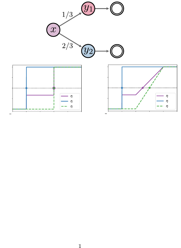
Perhaps surprisingly, there is in general no way to
determine the median of a return distribution based solely on the medians
at the successor states. To see this, consider a state
x
that leads to state
y
1
with probability
1
/3
and to state
y
2
with probability
2
/3
, with zero reward. The
following are two scenarios in which the median returns at
y
1
and
y
2
are the
same, but the median at x is different (see Figure 8.2):
63.
As usual, there might be multiple values of
z
for which
P
Z∼ν
(
Z ≤z
) = 0
.
5; recall that
F
−1
takes
the smallest such value.
Draft version.
242 Chapter 8
0.5 0.0 0.5 1.0 1.5 2.0
Return
0.00
0.25
0.50
0.75
1.00
Cumulative Probability
(x)
(y
1
)
(y
2
)
0.5 0.0 0.5 1.0 1.5
Return
0.00
0.25
0.50
0.75
1.00
Cumulative Probability
(x)
(y
1
)
(y
2
)
2.0
(c)(b)
(a)
Figure 8.2
Illustration of Example 8.10.
(a)
A Markov decision process in which state
x
leads to
states
y
1
and
y
2
with probability
1
/3
and
2
/3
, respectively.
(b)
Case 1, in which the median
of
η
(
x
) matches the median of
η
(
y
2
).
(c)
Case 2, in which the median of
η
(
x
) differs from
the median of η(y
2
).
Case 1. The return distributions at
y
1
and
y
2
are Dirac deltas at 0 and 1,
respectively, and these are also the medians of these distributions. The median
at x is also 1.
Case 2. The return distributions at
y
1
and
y
2
are a Dirac delta at 0 and the
uniform distribution on [0
.
5
,
1
.
5], respectively, and have the same medians as
in Case 1. However, the median at x is now 0.75. 4
Example 8.11
(
At-least functionals
)
.
For
ν ∈P
(
R
) and
z ∈R
, let us define
the at-least functional
ψ
≥z
(ν) = {P
Z∼ν
Z ≥z
> 0},
measuring whether
ν
assigns positive probability to values in [
z, ∞
). Now
consider a state
x
that deterministically leads to
y
, with no reward, and suppose
that there is a single action
a
available. The statement “it is possible to obtain a
return of at least 10 at state y” corresponds to
ψ
≥10
(η
π
(y)) = 1 . (8.7)
Draft version.

Statistical Functionals 243
If Equation 8.7 holds, can we deduce whether or not a return of at least 10 is
possible at state
x
? The answer is no. Suppose that
γ
= 0
.
9, and consider the
following two situations:
Case 1. η
π
(y) = δ
10
. Then ψ
≥10
(η
π
(y)) = 1, η
π
(x) = δ
9
and ψ
≥10
(η
π
(x)) = 0.
Case 2.
η
π
(
y
) =
δ
20
. Then
ψ
≥10
(
η
π
(
y
)) = 1 still. However,
η
π
(
x
) =
δ
18
and
ψ
≥10
(η
π
(x)) = 1. 4
What goes wrong in the examples above is that we do not have sufficient
information about the return distribution at the successor states to compute the
functional values for the return distribution of state
x
. Consequently, we cannot
use an iterative procedure to determine the functional values of
η
π
, at least not
without error.
As it turns out,
m
-moment sketches are somewhat special in being Bellman
closed. As the following theorem establishes, any sketch whose functionals
are expectations of functions must encode the same information as a moment
sketch.
Theorem 8.12.
Let
ψ
= (
ψ
1
, . . . , ψ
m
) be a sketch. Suppose that
ψ
is Bell-
man closed and that for each
i
= 1
, . . . , m
, there is a function
f
i
:
R →R
for
which
ψ
i
(ν) = E
Z∼ν
[ f
i
(Z)] .
Then,
ψ
is equivalent to the first
n
-moment functionals for some
n ≤m
, in
the sense that there are real-valued coefficients (
b
i j
) and (
c
i j
) such that for
any ν ∈P
ψ
(R) ∩P
m
(R),
ψ
i
(ν) =
n
X
j=1
b
i j
µ
j
(ν) + b
i0
, i = 1, . . . , m ;
µ
j
(ν) =
m
X
i=1
c
i j
ψ
i
(ν) + c
0 j
, j = 1, . . . , n . 4
The proof is somewhat lengthy and is given in Remark 8.2 at the end of the
chapter.
As a corollary, we may deduce that any sketch that can be expressed as
an invertible function of the first
m
moments is also Bellman closed. More
precisely, if
ψ
0
is a sketch that is an invertible transformation of the sketch
ψ
corresponding to the first
m
moments, say
ψ
0
=
h ◦ψ
, then
ψ
0
is Bellman closed
with corresponding Bellman operator
h ◦T
π
ψ
◦h
−1
. Thus, for example, we may
deduce that the sketch corresponding to the mean and variance functionals is
Bellman closed, since the mean and variance are expressible as an invertible
function of the mean and uncentered second moment. On the other hand, many
Draft version.
244 Chapter 8
other statistical functionals (including quantile functionals) are not covered by
Theorem 8.12. In the latter case, this is because there is no function
f
:
R →R
whose expectation for an arbitrary distribution
ν
recovers the
τ
th quantile of
ν
(Exercise 8.5). Still, as established in Example 8.10, quantile sketches are not
Bellman closed.
8.4 Statistical Functional Dynamic Programming
When a sketch
ψ
is not Bellman closed, we lack an operator
T
π
ψ
that emu-
lates the combination of the distributional Bellman operator and this sketch.
This precludes a dynamic programming approach that bootstraps its functional
value estimates directly from the previous estimates. However, approximate
dynamic programming with arbitrary statistical functionals is still possible if we
introduce an additional imputation step
ι
that reconstructs plausible probability
distributions from functional values. As we will now see, this allows us to apply
the distributional Bellman operator to the reconstructed distributions and then
extract the functional values of the resulting return function estimate.
Definition 8.13.
An imputation strategy for the sketch
ψ
:
P
ψ
(
R
)
→R
m
is a
function
ι
:
I
ψ
→P
ψ
(
R
). We say that it is exact if for any valid functional values
(s
1
, …, s
m
) ∈I
ψ
, we have
ψ
i
(ι(s
1
, …, s
m
)) = s
i
, i = 1, . . . , m .
Otherwise, we say that it is approximate.
By extension, we write
ι
(
s
)
∈P
ψ
(
R
)
X
for the return-distribution function
corresponding to the collection of functional values s ∈I
X
ψ
. 4
In other words, if
ι
is an exact imputation strategy for the sketch
ψ
=
(
ψ
1
, …, ψ
m
), then for any valid values
s
1
, …, s
m
of the functionals
ψ
1
, …, ψ
m
,
we have that
ι
(
s
1
, …, s
m
) is a probability distribution with the required values
under each functional. In a certain sense,
ι
is a pseudo-inverse to the vector-
valued map
ψ
:
ν 7→
(
ψ
1
(
ν
)
, …, ψ
m
(
ν
)). Note that a true inverse to
ψ
does not
exist, as ψ generally does not capture all aspects of the distribution ν.
Once an imputation strategy has been selected, it is possible to write down an
approximate dynamic programming algorithm for the functional values under
consideration. An abstract framework is given in Algorithm 8.1. In effect, such
an algorithm recursively computes the iterates
s
k+1
= ψ
T
π
ι(s
k
)
(8.8)
from an initial
s
0
∈I
X
ψ
. Procedures that implement the iterative process described
by Equation 8.8 are referred to as statistical functional dynamic programming
(SFDP) algorithms. When the sketch
ψ
is Bellman closed and its imputation
Draft version.

Statistical Functionals 245
strategy
ι
is exact, the sequence of iterates (
s
k
)
k≥0
converges to
ψ
(
η
π
), so long
as ψ is continuous (with respect to a Wasserstein metric).
Algorithm 8.1: Statistical functional dynamic programming
Algorithm parameters: statistical functionals ψ
1
, …, ψ
m
,
imputation strategy ι,
initial functional values
(s
i
(x))
m
i=1
: x ∈X
,
desired number of iterations K
for k = 1, . . . , K do
Impute distributions
η ←
ι(s
1
(x), …, s
m
(x)) : x ∈X
Apply distributional Bellman operator
˜η ←T
π
η
foreach state x ∈X do
for i = 1, . . . , m do
Update statistical functional
values
s
i
(x) ←ψ
i
(˜η(x))
end for
end foreach
end for
return
(s
i
(x))
m
i=1
: x ∈X
Example 8.14.
For the quantile functionals (
ψ
Q
τ
i
)
m
i=1
with
τ
i
=
2i−1
2m
for
i
=
1, …, m, an exact imputation strategy is
(q
1
, …, q
m
) 7→
1
m
m
X
i=1
δ
q
i
. (8.9)
This follows because the
2i−1
2m
-quantile of
1
m
m
P
i=1
δ
q
i
is precisely q
i
.
Note that when
τ
1
, . . . , τ
m
∈
(0
,
1) are arbitrary levels with quantile values
(
q
1
, . . . , q
m
), however, it is generally not true that Equation 8.9 is an exact
imputation strategy for the corresponding quantile functionals. 4
Example 8.15.
Categorical dynamic programming can be interpreted as an
SFDP algorithm. Indeed, the parameters
p
1
, …, p
m
found by the categorical
Draft version.

246 Chapter 8
projection correspond to the values of the following statistical functionals:
ψ
C
i
(ν) = E
Z∼ν
h
i
(ς
−1
m
(Z −θ
i
)
, i = 1, . . . , m (8.10)
where (
h
i
)
m
i=1
are the triangular and half-triangular kernels defining the cate-
gorical projection on (
θ
i
)
m
i=1
(Section 5.6). An exact imputation strategy in this
case is the function that returns the unique distribution supported on (
θ
i
)
m
i=1
that
matches the estimated functional values p
i
= ψ
C
i
(ν), i = 1, . . . , m:
(p
1
, . . . , p
m
) 7→
m
X
i=1
p
i
δ
θ
i
. 4
Mathematically, an exact imputation strategy always exists, because we
defined imputation strategies in terms of valid functional values. However, there
is no guarantee that an efficient algorithm exists to compute the application of
this strategy to arbitrary functional values. In practice, we may favor approx-
imate strategies with efficient implementations. For example, we may map
functional values to probability distributions from a representation
F
by opti-
mizing some notion of distance between functional values. The optimization
process may not yield an exact match in
F
(one may not even exist) but can
often be performed efficiently.
Example 8.16.
Let
ψ
c
1
, . . . , ψ
c
m
be the categorical functionals from Equation
8.10. Suppose we are given the corresponding functional values
p
1
, . . . , p
m
of a
probability distribution ν:
p
i
= ψ
c
i
(ν), i = 1, . . . , m .
An approximate imputation strategy for these functionals is to find the
n
-quantile
distribution (n possibly different from m)
ν
θ
=
1
n
n
X
i=1
δ
θ
i
that best fits p
i
according to the loss
L(θ) =
m
X
i=1
p
i
−ψ
c
i
(ν
θ
)
. (8.11)
Exercise 8.7 asks you to demonstrate that this strategy is approximate for
m >
2.
Although in this context, we know of an exact imputation strategy based on
categorical distributions, this illustrates that it is possible to impute distributions
from a different representation. 4
Draft version.
Statistical Functionals 247
8.5 Relationship to Distributional Dynamic Programming
In Chapter 5, we introduced distributional dynamic programming (DDP) as a
class of methods that operates over return-distribution functions. In fact, every
statistical functional dynamic programming is also a DDP algorithm (but not
the other way around; see Exercise 8.8). This relationship is established by
considering the implied representation
F = {ι(s) : s ∈I
ψ
}⊆P(R)
and the projection Π
F
= ι ◦ψ (see Figure 8.3).
η ˜η η
0
s s
0
T
π
Π
F
ψ
ι
ι
Figure 8.3
The interpretation of SFDP algorithms as distributional dynamic programming algo-
rithms. Traversing along the diagram from
η
to
η
0
corresponds to dynamic programming
implementing a projected Bellman operator, while the path from
s
to
s
0
corresponds to
statistical functional dynamic programming (SFDP).
From this correspondence, we may establish the relationship between Bell-
man closedness and the notion of a diffusion-free projection developed in
Chapter 5.
Proposition 8.17.
Let
ψ
be a Bellman-closed sketch. Then for any choice
of exact imputation strategy
ι
:
I
ψ
→P
ψ
(
R
), the projection operator Π
F
=
ιψ is diffusion-free. 4
Proof.
We may directly check the diffusion-free property (omitting parentheses
for conciseness):
Π
F
T
π
Π
F
= ιψT
π
ιψ
(a)
= ιT
π
ψ
ψιψ
(b)
= ιT
π
ψ
ψ
(a)
= ιψT
π
= Π
F
T
π
,
where steps marked (a) follow from the identity
ψT
π
=
T
π
ψ
ψ
, and (b) follows
from the identity ψιψ = ψ for any exact imputation strategy ι for ψ.
Imputation strategies formalize how one might interpret functional values
as parameters of a probability distribution. Naturally, the chosen imputation
Draft version.

248 Chapter 8
strategy affects the approximation artifacts from distributional dynamic pro-
gramming, the rate of convergence, and whether the algorithm converges at
all.
Compared with representation-based algorithms of the style introduced in
Chapter 5, working with statistical functionals allows us to design the projection
Π
F
in two separate pieces: a sketch
ψ
and an imputation strategy
ι
. In particular,
this makes it possible to learn statistical functionals that would be difficult to
directly capture in a probability distribution representation. As the next section
demonstrates, this allows us to create new kinds of distributional reinforcement
learning algorithms.
8.6 Expectile Dynamic Programming
Expectiles form a family of statistical functionals parameterized by a level
τ ∈
(0
,
1). They extend the notion of the mean of a distribution (
τ
= 0
.
5) similar
to how quantiles extend the notion of a median. Expectiles have classically
found application in econometrics and finance as a form of risk measure (see the
bibliographical remarks for further details). Based on the principles of statistical
functional dynamic programming, expectile dynamic programming
64
uses an
approximate imputation strategy in order to iteratively estimate the expectiles
of the return function.
Definition 8.18.
For a given
τ ∈
(0
,
1), the
τ
-expectile of a distribution
ν ∈
P
2
(R) is
ψ
e
τ
(ν) = arg min
z∈R
ER
τ
(z; ν) , (8.12)
where
ER
τ
(z; ν) = E
Z∼ν
|
{Z<z}
−τ|×(Z −z)
2
(8.13)
is the expectile loss. 4
The loss appearing in Definition 8.18 is strongly convex (Boyd and Vanden-
berghe 2004) and bounded below by 0. As a consequence, Equation 8.12 has a
unique minimizer for a given
τ
; this verifies that the corresponding expectile is
uniquely defined.
To understand the relationship to the mean functional and develop some
intuition for the statistical property than an expectile encodes, observe that the
mean of a distribution ν ∈P
2
(R) can be expressed as
µ
1
(ν) = arg min
z∈R
E
Z∼ν
[(Z −z)
2
] .
64.
The incremental analogue is called expectile temporal-difference learning (Rowland et al. 2019).
Draft version.

Statistical Functionals 249
Similar to how a quantile is derived from a loss that weights errors asymmetri-
cally (depending on whether the realization from
Z
is smaller or greater than
z
), the expectile loss for
τ ∈
(0
,
1) is the asymmetric version of the above. For
τ
greater than
1
/2
, one can think of the expectile as an “optimistic” summary of
the distribution – a value that emphasizes outcomes that are greater than the
mean. Conversely, for
τ
smaller than
1
/2
, the corresponding expectile is in a
sense “pessimistic.”
Expectile dynamic programming (EDP) estimates the values of a finite set
of expectile functionals with values 0
< τ
1
< ···< τ
m
<
1. For a distribution
ν ∈P
2
(R), let us write
e
i
= ψ
e
τ
i
(ν) .
Given the collection of expectile values
e
1
, …, e
m
, EDP uses an imputation
strategy that outputs an
n
-quantile probability distribution that approximately
has these expectile values.
65
The imputation strategy finds a suitable reconstruction by finding a solution to
a root-finding problem. To begin, this strategy outputs a
n
-quantile distribution
ˆν, with n possibly different from m:
ˆν =
1
n
n
X
j=1
δ
θ
j
.
Following Definition 8.13, for this imputation to be exact, the expectiles of
ˆν
at
τ
1
, . . . , τ
m
should be equal to e
1
, . . . , e
m
:
ψ
e
τ
i
(ˆν) = e
i
, i = 1, . . . , m .
This constraint implies that the derivatives of the expectile loss, instantiated
with τ
1
, . . . , τ
m
and evaluated with ˆν, should all be 0:
∂
z
ER
τ
i
z; ˆν
z=e
i
= 0, i = 1, . . . , m . (8.14)
Written out in full for the choice of ˆν above, these derivatives take the form
∂
z
ER
τ
i
z; ˆν
z=e
i
=
1
n
n
X
j=1
1
2
(e
i
−θ
j
)|
{θ
j
< e
i
}
−τ
i
|, i = 1, . . . , m .
An alternative to the root-finding problem expressed in Equation 8.14 is the
following optimization problem:
minimise
m
X
i=1
∂
z
ER
τ
i
z; ˆν
z=e
i
!
2
. (8.15)
65.
Of course, this particular form for the imputation strategy is a design choice; the reader is
invited to consider what other imputation strategies might be sensible here.
Draft version.
250 Chapter 8
A practical implementation of this imputation strategy therefore applies an opti-
mization algorithm to the objective in Equation 8.15, or a root-finding method
to Equation 8.14, viewed as functions of
θ
1
, …, θ
n
. Because the optimization
algorithm may return a solution that does not exactly satisfy Equation 8.14,
this method is an approximate (rather than exact) imputation strategy. It can
be used in the impute distributions step of Algorithm 8.1, yielding a dynamic
programming algorithm that aims to approximately learn return-distribution
expectiles. If the root-finding algorithm is always able to find
ˆν
exactly sat-
isfying Equation 8.14, then the imputation strategy is exact in this instance;
otherwise, it is approximate. A specific implementation is explored in detail in
Exercise 8.10.
8.7 Infinite Collections of Statistical Functionals
Thus far, our treatment of statistical functionals has focused on finite collec-
tions of statistical functionals – what we call a sketch. From a computational
standpoint, this is sensible since, to implement an SFDP algorithm, one needs
to be able to operate on individual functional values. On the other hand, in
Section 8.3, we saw that many sketches are not Bellman closed and must be
combined with an imputation strategy in order to perform dynamic program-
ming. An alternative, which we will study in greater detail in Chapter 10, is to
implicitly parameterize an infinite family of statistical functionals.
Many (though not all) infinite families of functionals provide a lossless
encoding of probability distributions and are consequently Bellman closed
– that is, knowing the values taken on by these functionals is equivalent to
knowing the distribution itself. We encode this property with the following
definition.
Definition 8.19.
Let Ψ be a set of statistical functionals. We say that Ψ char-
acterizes probability distributions over the real numbers if, for each
ν ∈P
(
R
),
there is a unique collection of functional values (ψ(ν) : ψ ∈Ψ). 4
The following families of statistical functionals all characterize probability
distributions over R.
The cumulative distribution function.
The functionals mapping distribu-
tions
ν
to the probabilities
P
Z∼ν
(
Z ≤z
), indexed by
z ∈R
. Closely related are
upper-tail probabilities,
ν 7→P
Z∼ν
(Z ≥z) ,
and the quantile functionals
ν 7→F
−1
ν
(τ) ,
indexed by τ ∈(0, 1).
Draft version.

Statistical Functionals 251
The characteristic function. Functionals of the form
ν 7→ E
Z∼ν
[e
iuZ
] ∈C ,
indexed by
u ∈R
(and where i
2
=
−
1). The corresponding collection of statistical
values is the characteristic function of ν, denoted χ
ν
.
Moments and cumulants.
The infinite collection of moment functionals
(
µ
p
)
∞
p=1
does not unconditionally characterize the distribution
ν
: there are distinct
distributions that have the same sequence of moments. However, if the sequence
of moments does not grow too quickly, uniqueness is restored. In particular, a
sufficient condition for uniqueness is that the underlying distribution
ν
has a
moment-generating function
u 7→ E
Z∼ν
[e
uZ
] ,
which is finite in an open neighborhood of
u
= 0; see Remark 8.3 for further
details. Under this condition, the moment-generating function itself also charac-
terizes the distribution, as does the cumulant-generating function, defined as
the logarithm of the moment-generating function,
u 7→log
E
Z∼ν
[e
uZ
]
.
The cumulants (
κ
p
)
∞
p=1
are defined through a power series expansion of the
cumulant-generating function
log
E
Z∼ν
[e
uZ
]
=
∞
X
p=1
κ
p
u
p
p!
.
Under the condition that the moment-generating function is finite in an open
neighborhood of the origin, the sequences of cumulants and moments are
determined by one another, and so the sequence of cumulants is another
characterization of the distribution under this condition.
Example 8.20. Consider the return-variable Bellman equation
G
π
(x, a)
D
= R + γG
π
(X
0
, A
0
) , X = x , A = a .
If for each
u ∈R
we apply the functional
ν 7→ E
Z∼ν
[
e
iuZ
] to the distribution of the
random variables on each side, we obtain the characteristic function Bellman
equation:
χ
η
π
(x,a)
(u) = E
π
[e
iu(R+γG
π
(X
0
,A
0
))
| X = x, A = a]
= E
π
e
iuR
| X = x, A = a
E
π
e
iγuG
π
(X
0
,A
0
)
| X = x, A = a
= χ
P
R
(·|x,a)
(u) E
π
χ
η
π
(X
0
,A
0
)
(γu) | X = x, A = a
.
Draft version.
252 Chapter 8
This is a different kind of distributional Bellman equation in which the addi-
tion of independent random variables corresponds to a multiplication of their
characteristic functions. The equation highlights that the characteristic function
of
ν
evaluated at
u
depends on the next-state characteristic functions evaluated
at
γu
. This shows that for a set
S ⊆R
, the sketch (
ν 7→χ
ν
(
u
) :
u ∈S
) cannot be
Bellman closed unless
S
is infinite or
S
=
{
0
}
. Exercise 8.12 asks you to give a
theoretical analysis of a dynamic programming approach based on characteristic
functions. 4
Another way to understand collections of statistical functionals that are
characterizing (in the sense of Definition 8.19) is to interpret them in light of
our definition of a probability distribution representation (Definition 5.2). Recall
that a representation
F
is a collection of distributions indexed by a parameter
θ:
F =
ν
θ
∈P (R) : θ ∈Θ
.
Here, the functional values associated with the set of statistical functionals Ψ
correspond to the (infinite-dimensional) parameter θ, so that
F
Ψ
= P(R) .
This clearly implies that
F
Ψ
is closed under the distributional Bellman operator
T
π
(Section 5.3) and hence that approximation-free distributional dynamic
programming is (mathematically) possible with F
Ψ
.
8.8 Moment Temporal-Difference Learning*
In Section 8.2, we introduced the
m
-moment Bellman operator, from which an
exact dynamic programming algorithm can be derived. A natural follow-up is to
apply the tools of Chapter 6 to derive an incremental algorithm for learning the
moments of the return-distribution function from samples. Here, an algorithm
that incrementally updates an estimate
M ∈R
X×A×m
of the
m
first moments of
the return function can be directly obtained through the unbiased estimation
approach, as the corresponding operator can be written as an expectation. Given
a sample transition (
x, a, r, x
0
, a
0
), the unbiased estimation approach yields the
update rule (for i = 1, . . . , m)
M(x, a, i) ←(1 −α)M(x, a, i) + α
i
X
j=0
γ
i−j
i
j
!
r
j
M(x
0
, a
0
, i − j)
, (8.16)
where again we take M(·, ·, 0) = 1 by convention.
Unlike the TD and CTD algorithms analyzed in Chapter 6, this algorithm is
derived from an operator,
T
π
(m)
, which is not a contraction in a supremum-norm
over states. As a result, the theory developed in Chapter 6 cannot immediately
Draft version.
Statistical Functionals 253
be applied to demonstrate convergence of this algorithm under appropriate
conditions. With some care, however, a proof is possible; we now give an
overview of what is needed.
The proof of Proposition 8.7 demonstrates that the behavior of
T
π
(m)
is closely
related to that of a contraction mapping. Specifically, the behavior of
T
π
(m)
in
updating the estimates of
i
th moments of returns is contractive if the lower
moment estimates are sufficiently close to their correct values. To turn these
observations into a proof of convergence, an inductive argument on the moments
being learnt must be made, as in the proof of Proposition 8.7. Further, the
approach of Chapter 6 needs to be extended to deal with a vanishing bias term
in the update to account for this “near-contractivity” of
T
π
(m)
; to this end one
may, for example, begin from the analysis of Bertsekas and Tsitsiklis (1996,
Proposition 4.5).
Before moving on, let us remark that in practice, we are likely to be interested
in centered moments such as the variance (m = 2); these take the form
E
π
h
∞
X
t=0
γ
t
R
t
−Q
π
(x, a)
m
X
0
= x, A
0
= a
i
,
These can be derived from their uncentered counterparts; for example, the vari-
ance of the return distribution
η
π
(
x, a
) is obtained from the first two uncentered
moments via Equation 8.2.
It is also possible to perform dynamic programming on centered moments
directly, as was shown in the context of the mean and variance in Section 5.4
(Exercise 8.14 asks you to derive the Bellman operators for the more general
case of the first m centered moments). Given in terms of state-action pairs, the
Bellman equation for the return variances
¯
M
π
(·, ·, 2) ∈R
X×A
is
¯
M
π
(x, a, 2) = Var
π
(R | X = x, A = a) + (8.17)
γ
2
Var
π
(Q
π
(X
0
, A
0
) | X = x, A = a) + E
π
[
¯
M
π
(X
0
, A
0
, 2) | X = x, A = a]
;
contrast with Equation 5.20.
One challenge with deriving an incremental algorithm for learning the vari-
ance directly is that unbiasedly estimating some of the variance terms on the
right-hand side requires multiple samples. For example, an unbiased estimator
of
Var
π
(Q
π
(X
0
, A
0
) | X = x, A = a)
in general requires two independent realizations of
X
0
, A
0
for a given source
state-action pair
x, a
. Consequently, unbiased estimation of the corresponding
operator application with a single transition is not feasible in this case. Despite
the fact that the first
m
centered and uncentered moments of a probability
Draft version.
254 Chapter 8
distribution can be recovered from one another, there is a distinct advantage
associated with working with uncentered moments when learning from samples.
8.9 Technical Remarks
Remark 8.1.
Theorem 8.12 illustrates how dynamic programming over func-
tional values must incur some approximation error, unless the underlying sketch
is Bellman closed. One way to avoid this error is to augment the state space
with additional information: for example, the return accumulated so far. We in
fact took this approach when optimizing the conditional value-at-risk (CVaR)
of the return in Chapter 7; in fact, risk measures are statistical functionals that
may also take on the value −∞ (see Definition 7.14). 4
Remark 8.2
(
Proof of Theorem 8.12
)
.
It is sufficient to consider a pair of
states,
x
and
y
, such that
x
deterministically transitions to
y
with reward
r
.
Because
ψ
is Bellman closed, we can identify an associated Bellman operator
T
π
ψ
. For a given return function
η
whose state-indexed collection of functional
values is
s
=
ψ
(
η
), let us write (
T
π
ψ
s
)
i
(
x
) for the
i
th functional value at state
x
,
for
i
= 1
, . . . , m
. By construction and definition of the operator
T
π
ψ
, (
T
π
ψ
s
)
i
(
x
) is a
function of the functional values at
y
as well as the reward
r
and discount factor
γ, and so we may write
(T
π
ψ
s)
i
(x) = g
i
r, γ, ψ
1
(η(y)), …, ψ
m
(η(y))
for some function
g
i
. We next argue that
g
i
is affine
66
in the inputs
ψ
1
(
η
(
y
))
, …, ψ
m
(
η
(
y
)). This is readily observed as each functional
ψ
1
, …, ψ
m
is
affine in its input distribution,
ψ
i
(αν + (1 −α)ν
0
) = E
Z∼αν+(1−α)ν
0
[ f
i
(Z)]
= α E
Z∼ν
[ f
i
(Z)] + (1 −α) E
Z∼ν
0
[ f
i
(Z)]
= αψ
i
(ν) + (1 −α)ψ
i
(ν
0
) ,
and
(T
π
ψ
s)
i
(x) = E
Z∼η(y)
[ f
i
(r + γZ)]
is also affine as a function of
η
. This affineness would be contradicted if
g
i
were
not also affine. Hence, there exist functions
β
i
:
R ×
[0
,
1)
→R
for
i
= 1
, …, m
66.
Recall that a function
h
:
M → M
0
between vector spaces
M
and
M
0
is affine if for
u
1
, u
2
∈ M
,
λ ∈(0, 1), we have h(λu
1
+ (1 −λ)u
2
) = λh(u
1
) + (1 −λ)h(u
2
).
Draft version.
Statistical Functionals 255
such that
g
i
r, γ, ψ
1
(η(y)), …, ψ
m
(η(y))
= β
0
(r, γ) +
m
X
i=1
β
i
(r, γ)ψ
i
(η(y)) ,
and therefore
E
Z∼η(y)
[ f
i
(r + γZ)] = E
Z∼η(y)
m
X
j=0
β
i
(r, γ) f
j
(Z)
,
where
f
0
(
z
) = 1. Taking
η
(
y
) to be a Dirac delta
δ
z
then gives the following
identity:
f
i
(r + γz) =
m
X
j=0
β
i
(r, γ) f
j
(z) .
We therefore have that the finite-dimensional function space spanned by
f
0
, f
1
, …, f
m
(where
f
0
is the constant function equal to 1) is closed under
translation (by
r ∈R
) and scaling (by
γ ∈
[0
,
1)). Engert (1970) shows that
the only finite-dimensional subspaces of measurable functions closed under
translation are contained in the span of finitely many functions of the form
z 7→z
exp
(
λz
), with
∈N
and
λ ∈C
. Since we further require closure under
scaling by
γ ∈
[0
,
1), we deduce that we must have
λ
= 0 in any such function,
and the subspace must be equal to the space spanned by the first
n
monomials
(and the constant function).
To conclude, since each monomial
z 7→z
i
for
i
= 1
, …, n
is expressible as a
linear combination of
f
0
, …, f
m
, the corresponding expectations
E
Z∼ν
[
Z
i
] are
expressible as linear combinations of the expectations
E
Z∼ν
[
f
j
(
Z
)], for any
distribution
ν
. The converse also holds, and so we conclude that the sketch
ψ
encodes the same distributional information as the first n moments. 4
Remark 8.3.
The question of whether a distribution is characterized by its
sequence of moments has been a subject of study in probability theory for
over a century. The sufficient condition on the moment-generating function
described in Section 8.8 means that the characteristic function of such a dis-
tribution can be written as a power series with scaled moments as coefficients,
ensuring uniqueness of the distribution; see, for example, Billingsley (2012)
for a detailed discussion. Lin (2017) gives a survey of known sufficient condi-
tions for characterization, as well as examples where characterization does not
hold. 4
8.10 Bibliographical Remarks
8.1.
Statistical functionals are a core notion in statistics; see, for example,
the classic text by van der Vaart (2000). In reinforcement learning, specific
Draft version.
256 Chapter 8
functionals such as moments, quantiles, and CVaR have been of interest for
risk-sensitive control (more on this in the bibliographical remarks of Chapter 7).
Chandak et al. (2021) consider the problem of off-policy Monte Carlo policy
evaluation of arbitrary statistical functionals of the return distribution.
8.2, 8.8.
Sobel (1982) gives a Bellman equation for return-distribution moments
for state-indexed value functions with deterministic policies. More recent work
in this direction includes that of Lattimore and Hutter (2012), Azar et al. (2013),
and Azar et al. (2017), who make use of variance estimates in combination with
Bernstein’s inequality to improve the efficiency of exploration algorithms, as
well as the work of White and White (2016), who use estimated return variance
to set trace coefficients in multistep TD learning methods. Sato et al. (2001),
Tamar et al. (2012), Tamar et al. (2013), and Prashanth and Ghavamzadeh
(2013) further develop methods for learning the variance of the return. Tamar
et al. (2016) show that the operator
T
π
(2)
is a contraction under a weighted
norm (see Exercise 8.4), develop an incremental algorithm with a proof of
convergence using the ODE method, and study both dynamic programming
and incremental algorithms under linear function approximation (the topic of
Chapter 9).
8.3–8.5.
The notion of Bellman closedness is due to Rowland et al. (2019),
although our presentation here is a revised take on the idea. The noted connec-
tion between Bellman closedness and diffusion-free representations and the
term “statistical functional dynamic programming” are new to this book.
8.6.
The expectile dynamic programming algorithm is new to this book but
is directly derived from expectile temporal-difference learning (Rowland et
al. 2019). Expectiles themselves were introduced by Newey and Powell (1987)
in the context of testing in econometric regression models, with the asymmetric
squared loss defining expectiles already appearing in Aigner et al. (1976).
Expectiles have since found further application as risk measures, particularly
within finance (Taylor 2008; Kuan et al. 2009; Bellini et al. 2014; Ziegel
2016; Bellini and Di Bernardino 2017). Our presentation here focuses on the
asymmetric squared loss, requiring a finite second-moment assumption, but an
equivalent definition allows expectiles to be defined for all distributions with a
finite first moment (Newey and Powell 1987).
8.7.
The study of characteristic functions in distributional reinforcement learn-
ing is due to Farahmand (2019), who additionally provides error propagation
analysis for the characteristic value iteration algorithm, in which value iteration
is carried out with characteristic function representations of return distributions.
Earlier, Mandl (1971) studied the characteristic function of the return in Markov
decision processes with deterministic immediate rewards and policies. Chow
et al. (2015) combine a state augmentation method (see Chapter 7) with an
Draft version.
Statistical Functionals 257
infinite-dimensional Bellman equation for CVaR values to learn a CVaR-optimal
policy. They develop an implementable version of the algorithm by tracking
finitely many CVaR values and using linear interpolation for the remainder, an
approach related to the imputation strategies described earlier in the chapter.
Characterization via the quantile function has driven the success of several large-
scale distributional reinforcement learning algorithms (Dabney et al. 2018a;
Yang et al. 2019), and is the subject of further study in Chapter 10.
8.11 Exercises
Exercise 8.1.
Consider the
m
-moment Bellman operator
T
π
(m)
(Definition 8.6).
For M ∈R
X×A×m
, define the norm
kMk
∞,max
= max
i∈{1,...,m}
sup
x∈X
a∈A
M(x, a, i).
By means of a counterexample, show that
T
π
(m)
is not a contraction mapping in
the metric induced by k·k
∞,max
. 4
Exercise 8.2.
Let
ε >
0. Determine a bound on the computational cost (in
O
(
·
)
notation) of performing iterative policy evaluation with the
m
-moment Bellman
operator to obtain an approximation
ˆ
M
π
such that
max
i∈{1,...,m}
sup
x∈X
a∈A
|
ˆ
M
π
(x, a, i) −M
π
(x, a, i)|< ε.
You may find it convenient to refer to the proof of Proposition 8.7. 4
Exercise 8.3.
Equation 5.2 gives the value function
V
π
as the solution of the
linear system of equations
V = r
π
+ γP
π
V.
Provide the analogous linear system for the moment function M
π
. 4
Exercise 8.4. The purpose of this exercise is to show that T
π
(2)
is a contraction
mapping on
R
X×A×2
in a weighted
L
∞
norm, as shown by Tamar et al. (2016).
Let
M ∈R
X×A×2
be a moment function estimate (specifically, for the first two
moments). For each α ∈(0, 1), define the α-weighted norm on R
X×A×2
by
kMk
α
= αkM
(1)
k
∞
+ (1 −α)kM
(2)
k
∞
,
where M
(i)
= M(·, ·, i) ∈R
X×A
. For any M, M
0
∈R
X×A×2
, show that
kT
π
(2)
(M−M
0
)k
α
≤αkγP
π
(M
(1)
− M
0
(1)
)k
∞
+ (1 −α)k2γC
r
P
π
(M
(1)
− M
0
(1)
) + γ
2
P
π
(M
(2)
− M
0
(2)
)k
∞
,
Draft version.
258 Chapter 8
where P
π
is the state-action transition operator, defined by
(P
π
Q)(x, a) =
X
(x
0
,a
0
)∈X×A
P
π
(x
0
|x, a)π(a
0
|x
0
)Q(x
0
, a
0
) ,
and C
r
is the diagonal reward operator
(C
r
Q)(x, a) = E[R |X = x, A = a]Q(x, a) .
Writing
λ ≥
0 for the Lipschitz constant of
C
r
P
π
with respect to the
L
∞
metric,
deduce that
kT
π
(2)
(M −M
0
)k
α
≤(αγ + 2(1 −α)γλ)kM
(1)
− M
0
(1)
k
∞
+ (1 −α)γ
2
kM
(2)
− M
0
(2)
k
∞
.
Hence, deduce that there exist parameters α ∈(0, 1), β ∈[0, 1) such that
kT
π
(2)
(M −M
0
)k
α
≤βkM −M
0
k
α
,
as required. 4
Exercise 8.5. Consider the median functional
ν 7→F
−1
ν
(0.5) .
Show that there does not exist a function f : R →R such that, for any ν ∈R,
E
Z∼ν
[ f (Z)] = F
−1
ν
(0.5) . 4
Exercise 8.6.
Consider the subset of probability distributions endowed with a
probability density
f
ν
. Repeat the preceding exercise for the differential entropy
functional
ν 7→−
Z
z∈R
f
ν
(z) log
f
ν
(z)
dz . 4
Exercise 8.7. For the imputation strategy of Example 8.16:
(i) show that for m = 2, the imputation strategy is exact, for any n ∈N
+
.
(ii)
show that for
m >
2, this imputation strategy is inexact. Hint. Find a
distribution ν for which ψ
c
i
(ι(p
1
, . . . , p
m
)) , p
i
, for some i = 1, . . . , m. 4
Exercise 8.8.
In Section 8.4, we argued that every statistical functional dynamic
programming algorithm is a distributional dynamic programming algorithm.
Explain why the converse is false. Under what circumstances may we favor
either an algorithm that operates on statistical functionals or one that operates
on probability distribution representations? 4
Exercise 8.9.
Consider an imputation strategy
ι
for a sketch
ψ
. We say the (
ψ, ι
)
pair is mean-preserving if, for any probability distribution ν ∈P
ψ
(R),
ν
0
= ιψ(ν)
Draft version.

Statistical Functionals 259
satisfies
E
Z∼ν
0
[Z] = E
Z∼ν
[Z] .
Show that in this case, the operator
ψ ◦T
π
◦ι
is also mean-preserving. 4
Exercise 8.10.
Using your favorite numerical computation software, implement
the expectile imputation strategy described in Section 8.6. Specifically:
(i)
Implement a procedure for approximately determining the expectile values
e
1
, . . . , e
m
of a given distribution. Hint. An incremental approach in the style
of quantile regression, or a binary search approach, will allow you to deal
with continuous distributions.
(ii)
Given a set of expectile values,
e
1
, . . . , e
m
, implement a procedure that
imputes an n-quantile distribution
1
n
n
X
i=1
δ
θ
i
by minimizing the objective given in Equation 8.15.
Test your implementation on discrete and continuous distributions, and compare
it with the best
m
-quantile approximation of those distributions. Is one method
better suited to discrete distributions than the other? More generally, when
might one method be preferred over the other? 4
Exercise 8.11.
Formulate a variant of expectile dynamic programming that
imputes
n
-quantile distributions and whose (possibly approximate) imputation
strategy is mean-preserving in the sense of Exercise 8.9. 4
Exercise 8.12
(*)
.
This exercise applies the line of reasoning from Chapter 4
to characteristic functions and is based on Farahmand (2019). For a probability
distribution ν, recall that its characteristic function χ
ν
is
χ
ν
(u) = E
Z∼ν
e
iuZ
.
Now, for p ∈[1, ∞), define the probability metric
d
1,p
(ν, ν
0
) =
Z
u∈R
|χ
ν
(u) −χ
ν
0
(u)|
|u|
p
du
and its supremum extension to return functions
d
1,p
(η, η
0
) = sup
(x,a)∈X×A
d
1,p
(η(x, a), η
0
(x, a)) .
(i) Determine a subset P
χ,p
(R) ⊆P(R) on which d
1,p
is a proper metric.
(ii)
Provide assumption(s) under which the return function
η
π
lies in
P
χ,p
(
R
).
Draft version.

260 Chapter 8
(iii)
Prove that for
p ≥
2, the distributional Bellman operator is a contraction
mapping in d
1,p
, with modulus γ
p−1
. 4
Exercise 8.13 (*). Consider the probability metric
d
2,2
(ν, ν
0
) =
Z
u∈R
χ
ν
(u) −χ
ν
0
(u)
2
u
2
du
1
/2
.
Show that
d
2,2
is the Cramér distance
2
. Hint. Use the Parseval–Plancherel
identity. 4
Exercise 8.14.
Let
m ∈N
+
. Derive a Bellman operator on
R
X×A×m
whose
unique fixed point
˜
M
π
is the collection of centered moments:
˜
M
π
(x, a, i) = E
h
G
π
(x, a) −Q
π
(x, a)
i
i
, i = 1, . . . , m . 4
Draft version.