7
Control
A superpressure balloon is a kind of aircraft whose altitude is determined by the
relative pressure between its envelope and the ambient atmosphere and which
can be flown high in the stratosphere. Like a submarine, a superpressure balloon
ascends when it becomes lighter and descends when it becomes heavier. Once
in flight, superpressure balloons are passively propelled by the winds around
them, so that their direction of travel can be influenced simply by changing their
altitude. This makes it possible to steer such a balloon in an energy-efficient
manner and have it operate autonomously for months at a time. Determining
the most efficient way to control the flight of a superpressure balloon by means
of altitude changes is an example of a control problem, the topic of this chapter.
In reinforcement learning, control problems are concerned with finding poli-
cies that achieve or maximize specified objectives. This is in contrast with
prediction problems, which are concerned with characterizing or quantifying
the consequences of following a particular policy. The study of control problems
involves not only the design of algorithms for learning optimal policies but
also the study of the behavior of these algorithms under different conditions,
such as when learning occurs one sample at a time (as per Chapter 6), when
noise is injected into the process, or when only a finite amount of data is made
available for learning. Under the distributional perspective, the dynamics of
control algorithms exhibit a surprising complexity. This chapter gives a brief
and necessarily incomplete overview of the control problem. In particular, our
treatment of control differs from most textbooks in that we focus on the distri-
butional component and for conciseness omit some traditional material such as
policy iteration and λ-return algorithms.
7.1 Risk-Neutral Control
The problem of finding a policy that maximizes the agent’s expected return is
called the risk-neutral control problem, as it is insensitive to the deviations of
Draft version. 197
198 Chapter 7
returns from their mean. We have already encountered risk-neutral control when
we introduced the Q-learning algorithm in Section 3.7. We begin this chapter
by providing a theoretical justification for this algorithm.
Problem 7.1
(Risk-neutral control)
.
Given an MDP (
X, A, ξ
0
, P
X
, P
R
) and
discount factor γ ∈[0, 1), find a policy π maximizing the objective function
J(π) = E
π
h
∞
X
t=0
γ
t
R
t
i
. 4
A solution π
∗
that maximizes J is called an optimal policy.
Implicit in the definition of risk-neutral control and our definition of a policy
in Chapter 2 is the fact that the objective
J
is maximized by a policy that only
depends on the current state: that is, one that takes the form
π : X→P(A) .
As noted in Section 2.2, policies of this type are more properly called sta-
tionary Markov policies and are but a subset of possible decision rules. With
stationary Markov policies, the action
A
t
is independent of the random vari-
ables
X
0
, A
0
, R
0
, . . . , X
t−1
, A
t−1
, R
t−1
given
X
t
. In addition, the distribution of
A
t
,
conditional on X
t
, is the same for all time indices t.
By contrast, history-dependent policies select actions on the basis on the
entire trajectory up to and including
X
t
(the history). Formally, a history-
dependent policy is a time-indexed collection of mappings
π
t
: (X×A×R)
t−1
×X→P(A) .
In this case, we have that
A
t
| (X
0:t
, A
0:t−1
, R
0:t−1
) ∼π
t
(· | X
0
, A
0
, R
0
, . . . , A
t−1
, R
t−1
, X
t
) . (7.1)
When clear from context, we omit the time subscript to
π
t
and write
P
π
,
E
π
,
G
π
, and
η
π
to denote the joint distribution, expectation, return-variable function,
and return-distribution function implied by the generative equations but with
Equation 7.1 substituting the earlier definition from Section 2.2. We write
π
ms
for the space of stationary Markov policies and
π
h
for the space of history-
dependent policies.
It is clear that every stationary Markov policy is a history-dependent policy,
though the converse is not true. In risk-neutral control, however, the added
degree of freedom provided by history-dependent policies is not needed to
achieve optimality; this is made formal by the following proposition (recall that
a policy is deterministic if it always selects the same action for a given state or
history).
Draft version.

Control 199
Proposition 7.2.
Let
J
(
π
) be as in Problem 7.1. There exists a determinis-
tic stationary Markov policy π
∗
∈π
ms
such that
J(π
∗
) ≥J(π) ∀π ∈π
h
. 4
Proposition 7.2 is a central result in reinforcement learning – from a computa-
tional point of view, for example, it is easier to deal with deterministic policies
(there are finitely many of them) than stochastic policies. Remark 7.1 discusses
some other beneficial consequences of Proposition 7.2. Its proof involves a
surprising amount of detail; we refer the interested reader to Puterman (2014,
Section 6.2.4).
7.2 Value Iteration and Q-Learning
The main consequence of Proposition 7.2 is that when optimizing the risk-
neutral objective, we can restrict our attention to deterministic stationary Markov
policies. In turn, this makes it possible to find an optimal policy
π
∗
by computing
the optimal state-action value function Q
∗
, defined as
Q
∗
(x, a) = sup
π∈π
ms
E
π
h
∞
X
t=0
γ
t
R
t
| X = x, A = a
i
. (7.2)
Just as the value function
V
π
for a given policy
π
satisfies the Bellman equation,
Q
∗
satisfies the Bellman optimality equation:
Q
∗
(x, a) = E
R + γ max
a
0
∈A
Q
∗
(X
0
, a
0
) | X = x, A = a
. (7.3)
The optimal state-action value function describes the expected return obtained
by acting so as to maximize the risk-neutral objective when beginning from
the state-action pair (
x, a
). Intuitively, we may understand Equation 7.3 as
describing this maximizing behavior recursively. While there might be multiple
optimal policies, they must (by definition) achieve the same objective value in
Problem 7.1. This value is
E
π
[V
∗
(X
0
)] ,
where V
∗
is the optimal value function:
V
∗
(x) = max
a∈A
Q
∗
(x, a) .
Given
Q
∗
, an optimal policy is obtained by acting greedily with respect to
Q
∗
–
that is, choosing in state x any action a that maximizes Q
∗
(x, a).
Value iteration is a procedure for finding the optimal state-action value
function
Q
∗
iteratively, from which
π
∗
can then be recovered by choosing
actions that have maximal state-action values. In Chapter 5, we discussed a
Draft version.
200 Chapter 7
procedure for computing
V
π
based on repeated applications of the Bellman
operator
T
π
. Value iteration replaces the Bellman operator
T
π
in this procedure
with the Bellman optimality operator
(T Q)(x, a) = E
π
R + γ max
a
0
∈A
Q(X
0
, a
0
) | X = x, A = a
. (7.4)
Let us define the L
∞
norm of a state-action value function Q ∈R
X×A
as
kQk
∞
= sup
x∈X,a∈A
|Q(x, a)|.
As the following establishes, the Bellman optimality operator is a contraction
mapping in this norm.
Lemma 7.3.
The Bellman optimality operator
T
is a contraction in
L
∞
norm
with modulus γ. That is, for any Q, Q
0
∈R
X×A
,
kT Q −T Q
0
k
∞
≤γkQ −Q
0
k
∞
. 4
Corollary 7.4.
The optimal state-action value function
Q
∗
is the only value
function that satisfies the Bellman optimality equation. Further, for any
Q
0
∈
R
X×A
, the sequence (
Q
k
)
k≥0
defined by
Q
k+1
=
T Q
k
(for
k ≥
0) converges to
Q
∗
. 4
Corollary 7.4 is an immediate consequence of Lemma 7.3 and Proposition
4.7. Before we give the proof of Lemma 7.3, it is instructive to note that despite
a visual similarity and the same contractive property in supremum norm, the
optimality operator behaves somewhat differently from the fixed-policy operator
T
π
, defined for state-action value functions as
(T
π
Q)(x, a) = E
π
R + γQ(X
0
, A
0
) | X = x, A = a] , (7.5)
where conditional on the random variables (
X
=
x, A
=
a, R, X
0
), we have
A
0
∼
π
(
· | X
0
). In the context of this chapter, we call
T
π
a policy evaluation operator.
Such an operator is said to be affine: for any two Q-functions
Q, Q
0
and
α ∈
[0
,
1],
it satisfies
T
π
(αQ + (1 −α)Q
0
) = αT
π
Q + (1 −α)T
π
Q
0
. (7.6)
Equivalently, the difference between T
π
Q and T
π
Q
0
can be expressed as
T
π
Q −T
π
Q
0
= γP
π
(Q −Q
0
) .
The optimality operator, on the other hand, is not affine. While affine operators
can be analyzed almost as if they were linear,
54
the optimality operator is
generally a nonlinear operator. As such, its analysis requires a slightly different
approach.
54. Consider the proof of Proposition 4.4.
Draft version.

Control 201
Proof of Lemma 7.3.
The proof relies on a special property of the maximum
function. For f
1
, f
2
: A→R, it can be shown that
max
a∈A
f
1
(a) −max
a∈A
f
2
(a)
≤max
a∈A
f
1
(a) − f
2
(a)
.
Now let
Q, Q
0
∈R
X×A
, and fix
x ∈X, a ∈A
. Let us write
E
xa,π
[
·
] =
E
π
[
· | X
=
x, A = a]. By linearity of expectations, we have
|(T Q)(x, a) −(T Q
0
)(x, a)|=
E
xa,π
[R + γ max
a
0
∈A
Q(X
0
, a
0
) −R −γ max
a
0
∈A
Q
0
(X
0
, a
0
)]
=
E
xa,π
[γ max
a
0
∈A
Q(X
0
, a
0
) −γ max
a
0
∈A
Q
0
(X
0
, a
0
)]
= γ
E
xa,π
[max
a
0
∈A
Q(X
0
, a
0
) −max
a
0
∈A
Q
0
(X
0
, a
0
)]
≤γ E
xa,π
|max
a
0
∈A
Q(X
0
, a
0
) −max
a
0
∈A
Q
0
(X
0
, a
0
)|
≤γ E
xa,π
max
a
0
∈A
|Q(X
0
, a
0
) −Q
0
(X
0
, a
0
)|
≤γ max
(x
0
,a
0
)∈X×A
|Q(x
0
, a
0
) −Q
0
(x
0
, a
0
)|
= γkQ −Q
0
k
∞
.
Since the bound holds for any (x, a) pair, it follows that
kT Q −T Q
0
k
∞
≤γkQ −Q
0
k
∞
.
Corollary 7.5.
For any initial state-action value function
Q
0
∈R
X×A
, the
sequence of iterates Q
k+1
= T Q
k
converges to Q
∗
in the L
∞
norm. 4
We can use the unbiased estimation method of Section 6.2 to derive an
incremental algorithm for learning
Q
∗
, since the contractive operator
T
is
expressible as an expectation over a sample transition. Given a realization
(x, a, r, x
0
), we construct the sample target
r + γ max
a
0
∈A
Q(x
0
, a
0
) .
We then incorporate this target to an update rule to obtain the Q-learning
algorithm first encountered in Chapter 3:
Q(x, a) ←(1 −α)Q(x, a) + α(r + γ max
a
0
∈X
Q(x
0
, a
0
)) .
Under appropriate conditions, the convergence of Q-learning to
Q
∗
can be
established with Lemma 7.3 and a suitable extension of the analysis of Chapter
6 to the space of action-value functions.
Draft version.
202 Chapter 7
7.3 Distributional Value Iteration
Analogous to value iteration, we can devise a distributional dynamic pro-
gramming procedure for the risk-neutral control problem; such a procedure
determines an approximation to the return function of an optimal policy. As
we will see, in some circumstances, this can be accomplished without compli-
cations, giving some theoretical justification for the distributional algorithm
presented in Section 3.7.
As in Chapter 5, we perform distributional dynamic programming by imple-
menting the combination of a projection step with a distributional optimality
operator.
55
Because it is not possible to “directly maximize” a probability
distribution, we instead define the operator via a greedy selection rule G.
We can view the expected-value optimality operator
T
as substituting the
expectation over the next-state action
A
0
in Equation 7.5 by a maximization
over
a
0
. As such, it can be rewritten as a particular policy evaluation operator
T
π
whose policy
π
depends on the operand
Q
; the mapping from
Q
to
π
is what
we call a greedy selection rule.
Definition 7.6.
A greedy selection rule is a mapping
G
:
R
X×A
→π
ms
with the
property that for any Q ∈R
X×A
, G(Q) is greedy with respect to Q. That is,
G(Q)(a | x) > 0 =⇒ Q(x, a) = max
a
0
∈A
Q(x, a
0
) .
We extend
G
to return functions by defining, for
η ∈P
1
(
R
)
X×A
, the induced
state-action value function
Q
η
(x, a) = E
Z∼η(x,a)
[Z] ,
and then letting
G(η) = G(Q
η
) . 4
A greedy selection rule may produce stochastic policies, for example when
assigning equal probability to two equally valued actions. However, it must
select actions that are maximally valued according to
Q
. Given a greedy
selection rule, we may rewrite the Bellman optimality operator as
T Q = T
G(Q)
Q . (7.7)
In the distributional setting, we must make explicit the dependency of the oper-
ator on the greedy selection rule
G
. Mirroring Equation 7.7, the distributional
55.
As before, this implementation is at its simplest when there are finitely many possible states,
actions, and rewards, and the projection step can be computed efficiently. Alternatives include a
sample-based approach and, as we will see in Chapter 9, function approximation.
Draft version.
Control 203
η η
0
Q Q
0
Π
F
T
G
T
Figure 7.1
When the projection step Π
F
is mean-preserving, distributional value iteration produces
the same sequence of state-action value functions as standard value iteration.
Bellman optimality operator derived from G is
T
G
η = T
G(η)
η .
We will see that, unlike the expected-value setting, different choices of the
greedy selection rule result in different operators with possibly different dynam-
ics – we thus speak of the distributional Bellman optimality operators, in the
plural.
Distributional value iteration algorithms combine a greedy selection rule G
and a projection step (described by the operator Π
F
and implying a particular
choice of representation
F
) to compute an approximate optimal return function.
Given some initial return function
η
0
∈F
X×A
, distributional value iteration
implements the iterative procedure
η
k+1
= Π
F
T
G(η
k
)
η
k
. (7.8)
In words, distributional value iteration selects a policy that at each state
x
is
greedy with respect to the expected values of
η
k
(
x, ·
) and computes the return
function resulting from a single step of distributional dynamic programming
with that policy.
The induced value function
Q
η
k
plays an important role in distributional
value iteration as it is used to derive the greedy policy
π
k
=
G
(
η
k
). When Π
F
is
mean-preserving (Section 5.11),
Q
η
k
behaves as if it had been computed from
standard value iteration (Figure 7.1). That is,
Q
η
k+1
= T Q
η
k
.
By induction, distributional value iteration then produces the same sequence of
state-action value functions as regular value iteration. That is, given the initial
condition
Q
0
(x, a) = E
Z∼η
0
(x,a)
[Z] , (x, a) ∈X×A,
Draft version.
204 Chapter 7
and the recursion
Q
k+1
= T Q
k
,
we have
Q
η
k
= Q
k
, for all k ≥0 .
As a consequence, these two processes also produce the same greedy policies:
π
k
= G(Q
k
) .
In the following section, we will use this equivalence to argue that distributional
value iteration finds an approximation to an optimal return function. When Π
F
is not mean-preserving, however,
Q
η
k
may deviate from
Q
k
. If that is the case,
the greedy policy
π
k
is likely to be different from
G
(
Q
k
), and distributional
value iteration may converge to the return function of a suboptimal policy. We
discuss this point in Remark 7.2.
Before moving on, let us remark on an alternative procedure for approximat-
ing an optimal return function. This procedure first performs standard value
iteration to obtain an approximation
ˆ
Q
to
Q
∗
. A greedy policy
ˆπ
is then extracted
from
ˆ
Q
. Finally, distributional dynamic programming is used to approximate
the return function
η
ˆπ
. If
ˆπ
is an optimal policy, this directly achieves our stated
aim and suggests doing away with the added complexity of distributional value
iteration. In larger problems, however, it is difficult or undesirable to wait until
Q
∗
has been determined before learning or computing the return function, or it
may not be possible to decouple value and return predictions. In these situations,
it is sensible to consider distributional value iteration.
7.4 Dynamics of Distributional Optimality Operators
In this section and the next, we analyze the behavior of distributional optimality
operators; recall from Section 7.3 that there is one such operator for each choice
of greedy selection rule
G
, in contrast to non-distributional value iteration.
Combined with a mean-preserving projection, our analysis also informs the
behavior of distributional value iteration. As we will see, even in the absence of
approximation due to a finite-parameter representation, distributional optimality
operators exhibit complex behavior.
Thus far, we have analyzed distributional dynamic programming algorithms
by appealing to contraction mapping theory. Demonstrating that an opera-
tor is a contraction provides a good deal of understanding about algorithms
implementing its repeated application: they converge at a geometric rate to the
operator’s fixed point (when such a fixed point exists). Unfortunately, distri-
butional optimality operators are not contraction mappings, as the following
shows.
Draft version.
Control 205
η T
G
η η
∗
x, · γε ±γ γε
y, a −ε ε ε
y, b ±1 ±1 ±1
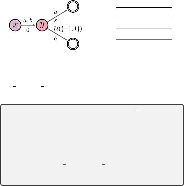
Figure 7.2
Left
: A Markov decision process for which no distributional Bellman optimality operator
is a contraction mapping. Right: The optimal return-distribution function η
∗
and initial
return-distribution function
η
used in the proof of Proposition 7.7 (expressed in terms of
their support). Given a
c
-homogeneous probability metric
d
, the proof chooses
ε
so as to
make d(T
G
η, η
∗
) > d(η, η
∗
).
Proposition 7.7.
Consider a probability metric
d
and let
d
be its supremum
extension. Suppose that for any z, z
0
∈R,
d(δ
z
, δ
z
0
) < ∞.
If
d
is
c
-homogeneous, there exist a Markov decision process and two
return-distribution functions
η, η
0
such that for any greedy selection rule
G
and any discount factor γ ∈(0, 1],
d(T
G
η, T
G
η
0
) > d(η, η
0
) . (7.9)
4
Proof.
Consider an MDP with two nonterminal states
x, y
and two actions
a, b
(Figure 7.2). From state
x
, all actions transition to state
y
and yield no reward.
In state
y
, action
a
results in a reward of
ε >
0, while action
b
results in a reward
that is
−
1 or 1 with equal probability; both actions are terminal. We will argue
that ε can be chosen to make T
G
satisfy Equation 7.9.
First note that any optimal policy must choose action
a
in state
y
, and all
optimal policies share the same return-distribution function
η
∗
. Consider another
return-distribution function
η
that is equal to
η
∗
at all state-action pairs except
that
η
(
y, a
) =
δ
−ε
(Figure 7.2, right). This implies that the greedy selection rule
must select b in y, and hence
(T
G
η)(x, a) = (T
G
η)(x, b) = (b
0,γ
)
#
η(y, b) = (b
0,γ
)
#
η
∗
(y, b) .
Because both actions are terminal from y, we also have that
(T
G
η)(y, a) = η
∗
(y, a)
Draft version.

206 Chapter 7
(T
G
η)(y, b) = η
∗
(y, b).
Let us write
ν
=
1
2
δ
−1
+
1
2
δ
1
for the reward distribution associated with (
y, b
).
We have
d(η, η
∗
) = d
η(y, a), η
∗
(y, a)
= d(δ
−ε
, δ
ε
) , (7.10)
and
d(T
G
η, T
G
η
∗
) = d
(T
G
η)(x, a), (T
G
η
∗
)(x, a)
= d
(b
0,γ
)
#
η
∗
(y, b), (b
0,γ
)
#
η
∗
(y, a)
= γ
c
d(ν, δ
ε
) , (7.11)
where the last line follows by
c
-homogeneity (Definition 4.22). We will show
that for sufficiently small ε > 0, we have
d(ν, δ
ε
) > γ
−c
d(δ
−ε
, δ
ε
) ,
from which the result follows by Equations 7.10 and 7.11. To this end, note that
d(δ
−ε
, δ
ε
) = ε
c
d(δ
−1
, δ
1
). (7.12)
Since
d
is finite for any pair of Dirac deltas, we have that
d
(
δ
−1
, δ
1
)
< ∞
and so
lim
ε→0
d(δ
−ε
, δ
ε
) = 0 . (7.13)
On the other hand, by the triangle inequality we have
d(ν, δ
ε
) + d(δ
0
, δ
ε
) ≥d(ν, δ
0
) > 0 , (7.14)
where the second inequality follows because
ν
and
δ
0
are different distributions.
Again by c-homogeneity of d, we deduce that
lim
ε→0
d(δ
0
, δ
ε
) = 0 ,
and hence
lim inf
ε→0
d(ν, δ
ε
) ≥d(ν, δ
0
) > 0 .
Therefore, for ε > 0 sufficiently small, we have
d(ν, δ
ε
) > γ
−c
d(δ
−ε
, δ
ε
) ,
as required.
Proposition 7.7 establishes that for any metric
d
that is sufficiently well
behaved to guarantee that policy evaluation operators are contraction mappings
(finite on bounded-support distributions,
c
-homogeneous), optimality operators
are not generally contraction mappings with respect to
d
. As a consequence,
Draft version.

Control 207
we cannot directly apply the tools of Chapter 4 to characterize distributional
optimality operators. The issue, which is implied in the proof above, is that it is
possible for distributions to have similar expectations yet differ substantially,
for example, in their variance.
With a more careful line of reasoning, we can still identify situations in which
the iterates
η
k+1
=
T
G
η
k
do converge. The most common scenario is when there
is a unique optimal policy. In this case, the analysis is simplified by the existence
of an action gap in the optimal value function.
56
Definition 7.8.
Let
Q ∈R
X×A
. The action gap at a state
x
is the difference
between the highest-valued and second highest-valued actions:
gap(Q, x) = min
Q(x, a
∗
) −Q(x, a) : a
∗
, a ∈A, a
∗
, a, Q(x, a
∗
) = max
a
0
∈A
Q(x, a
0
)
.
The action gap of Q is the smallest gap over all states:
gap(Q) = min
x∈X
gap(Q, x) .
By extension, the action gap for a return function η is
gap(η) = min
x∈X
gap(Q
η
, x) , Q
η
(x, a) = E
Z∼η(x,a)
[Z] . 4
Definition 7.8 is such that if two actions are optimal at a given state, then
gap
(
Q
∗
) = 0. When
gap
(
Q
∗
)
>
0, however, there is a unique action that is optimal
at each state (and vice versa). In this case, we can identify an iteration
K
from
which
G
(
η
k
) =
π
∗
for all
k ≥K
. From that point on, any distributional optimality
operator reduces to the
π
∗
evaluation operator, which enjoys now-familiar
convergence guarantees.
Theorem 7.9.
Let
T
G
be the distributional Bellman optimality operator
instantiated with a greedy selection rule
G
. Suppose that there is a unique
optimal policy
π
∗
and let
p ∈
[1
, ∞
]. Under Assumption 4.29(
p
) (well-
behaved reward distributions), for any initial return-distribution function
η
0
∈P (R), the sequence of iterates defined by
η
k+1
= T
G
η
k
converges to η
π
∗
with respect to the metric w
p
. 4
Theorem 7.9 is stated in terms of supremum
p
-Wasserstein distances for
conciseness. Following the conditions of Theorem 4.25 and under a different
set of assumptions, we can of course also establish the convergence in, say, the
supremum Cramér distance.
56. Example 6.1 introduced an update rule that increases this action gap.
Draft version.

208 Chapter 7
Corollary 7.10.
Suppose that Π
F
is a mean-preserving projection for some
representation
F
and that there is a unique optimal policy
π
∗
. If Assump-
tion 5.22(
w
p
) holds and Π
F
is a nonexpansion in
w
p
, then under the conditions
of Theorem 7.9, the sequence
η
k+1
= Π
F
T
G
η
k
produced by distributional value iteration converges to the fixed point
ˆη
π
∗
= Π
F
T
π
∗
ˆη
π
∗
. 4
Proof of Theorem 7.9.
As there is a unique optimal policy, it must be that the
action gap of
Q
∗
is strictly greater than zero. Fix
ε
=
1
2
gap
(
Q
∗
). Following the
discussion of the previous section, we have that
Q
η
k+1
= T Q
η
k
.
Because
T
is a contraction in
L
∞
norm, we know that there exists a
K
ε
∈N
after
which
kQ
η
k
−Q
∗
k
∞
< ε ∀k ≥K
ε
. (7.15)
For a fixed
x
, let
a
∗
be the optimal action in that state. From Equation 7.15, we
deduce that for any a , a
∗
,
Q
η
k
(x, a
∗
) ≥Q
∗
(x, a
∗
) −ε
≥Q
∗
(x, a) + gap(Q
∗
) −ε
> Q
η
k
(x, a) + gap(Q
∗
) −2ε
= Q
η
k
(x, a) .
Thus, the greedy action in state
x
after time
K
ε
is the optimal action for that
state. Thus, G(η
k
) = π
∗
for k ≥K
ε
and
η
k+1
= T
π
∗
η
k
k ≥K
ε
.
We can treat
η
K
ε
as a new initial condition
η
0
0
, and apply Proposition 4.30 to
conclude that η
k
→η
π
∗
.
In Section 3.7, we introduced the categorical Q-learning algorithm in terms
of a deterministic greedy policy. Generalized to an arbitrary greedy selection
rule G, categorical Q-learning is defined by the update
η(x, a) ←(1 −α)η(x, a) + α
X
a
0
∈A
G(η)(a
0
| x
0
)
Π
c
(b
r,γ
)
#
η
x
0
, a
0
.
Draft version.
Control 209
Because the categorical projection is mean-preserving, its induced state-value
function follows the update
Q
η
(x, a) ←(1 −α)η(x, a) + α
X
a
0
∈A
G(η)(a
0
| x
0
)
r + γQ
η
(x
0
, a
0
)
| {z }
r+γ max
a
0
∈A
Q
η
(x
0
,a
0
)
.
Using the tools of Chapter 6, one can establish the convergence of categorical
Q-learning under certain conditions, including the assumption that there is a
unique optimal policy
π
∗
. The proof essentially combines the insight that, under
certain conditions, the sequence of greedy policies tracked by the algorithm
matches that of Q-learning and hence eventually converges to
π
∗
, at which point
the algorithm is essentially performing categorical policy evaluation of
π
∗
. The
actual proof is somewhat technical; we omit it here and refer the interested
reader to Rowland et al. (2018).
7.5 Dynamics in the Presence of Multiple Optimal Policies*
In the value-based setting, it does not matter which greedy selection rule is used
to represent the optimality operator: By definition, any greedy selection rule
must be equivalent to directly maximizing over
Q
(
x, ·
). In the distributional
setting, however, different rules usually result in different operators. As a con-
crete example, compare the rule “among all actions whose expected value is
maximal, pick the one with smallest variance” to “assign equal probability to
actions whose expected value is maximal.”
Theorem 7.9 relies on the fact that, when there is a unique optimal policy
π
∗
, we can identify a time after which the distributional optimality operator
behaves like a policy evaluation operator. When there are multiple optimal
policies, however, the action gap of the optimal value function
Q
∗
is zero and
the argument cannot be used. To understand why this is problematic, it is useful
to write the iterates (η
k
)
k≥0
more explicitly in terms of the policies π
k
= G(η
k
):
η
k+1
= T
π
k
η
k
= T
π
k
T
π
k−1
η
k−1
= T
π
k
···T
π
0
η
0
. (7.16)
When the action gap is zero, the sequence of policies
π
k
, π
k+1
, . . .
may con-
tinue to vary over time, depending on the greedy selection rule. Although all
optimal actions have the same optimal value (guaranteeing the convergence
of the expected values to
Q
∗
), they may correspond to different distributions.
Thus, distributional value iteration – even with a mean-preserving projection –
may mix together the distribution of different optimal policies. Even if (
π
k
)
k≥0
converges, the policy it converges to may depend on initial conditions (Exercise
7.5). In the worst case, the iterates (
η
k
)
k≥0
might not even converge, as the
following example shows.
Draft version.
210 Chapter 7
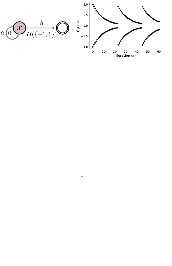
Figure 7.3
Left
: A Markov decision process in which the sequence of return function estimates
(
η
k
)
k≥0
does not converge (Example 7.11).
Right
: The return-distribution function esti-
mate at (
x, a
) as a function of
k
and beginning with
c
0
= 1. At each
k
, the pair of dots
indicates the support of the distribution.
Example 7.11
(Failure to converge)
.
Consider a Markov decision process with
a single nonterminal state
x
and two actions,
a
and
b
(Figure 7.3, left). Action
a
gives a reward of 0 and leaves the state unchanged, while action
b
gives a
reward of
−
1 or 1 with equal probability and leads to a terminal state. Note that
the expected return from taking either action is 0.
Let
γ ∈
(0
,
1)
.
We will exhibit a sequence of return function estimates (
η
k
)
k≥0
that is produced by distributional value iteration and does not have a limit. We
do so by constructing a greedy selection rule that achieves the desired behavior.
Suppose that
η
0
(x, b) =
1
2
(δ
−1
+ δ
1
) .
For any initial parameter c
0
∈R, if
η
0
(x, a) =
1
2
(δ
−c
0
+ δ
c
0
) ,
then by induction, there is a sequence of scalars (c
k
)
k≥0
such that
η
k
(x, a) =
1
2
(δ
−c
k
+ δ
c
k
) ∀k ∈N . (7.17)
This is because
η
k+1
(x, a) = (b
0,γ
)
#
η
k
(x, a) or η
k+1
(x, a) = (b
0,γ
)
#
η
k
(x, b), k ≥0 .
Define the following greedy selection rule: at iteration
k
+ 1, choose
a
if
c
k
≥
1
10
;
otherwise, choose b. With some algebra, this leads to the recursion (k ≥0)
c
k+1
=
(
γ if c
k
<
1
10
,
γc
k
otherwise.
Over a period of multiple iterations, the estimate
η
k
(
x, a
) exhibits cyclical
behavior (Figure 7.3, right). 4
Draft version.

Control 211
The example illustrates how, without additional constraints on the greedy
selection rule, it is not possible to guarantee that the iterates converge. However,
one can prove a weaker result based on the fact that only optimal actions must
eventually be chosen.
Definition 7.12.
For a given Markov decision process
M
, the set of nonstation-
ary Markov optimal return-distribution functions is
η
nmo
= {η
¯π
: ¯π = (π
k
)
k≥0
, π
k
∈π
ms
is optimal for M, ∀k ∈N}. 4
In particular, any history-dependent policy
¯π
satisfying the definition above is
also optimal for M.
Theorem 7.13.
Let
T
G
be a distributional Bellman optimality operator
instantiated with some greedy selection rule, and let
p ∈
[1
, ∞
]. Under
Assumption 4.29(
p
), for any initial condition
η
0
∈P
p
(
R
)
X
the sequence
of iterates η
k+1
= T
G
η
k
converges to the set η
nmo
, in the sense that
lim
k→∞
inf
η∈η
nmo
w
p
(η, η
k
) = 0. 4
Proof.
Along the lines of the proof of Theorem 7.9, there must be a time
K ∈N
after which the greedy policies
π
k
,
k ≥K
are optimal. For
l ∈N
+
, let us construct
the history-dependent policy
¯π = π
K+l−1
, π
K+l−2
, . . . , π
K+1
, π
K
, π
∗
, π
∗
, . . . ,
where
π
∗
is some stationary Markov optimal policy. Denote the return of this
policy from the state-action pair (
x, a
) by
G
¯π
(
x, a
) and its return-distribution
function by
η
¯π
. Because
¯π
is an optimal policy, we have that
η
¯π
∈η
nmo
. Let
G
k
be an instantiation of
η
k
, for each
k ∈N
. Now for a fixed
x ∈X
,
a ∈A
,
let (
X
t
, A
t
, R
t
)
l
t=0
be the initial segment of a random trajectory generated by
following
¯π
beginning with
X
0
=
x, A
0
=
a
. More precisely, for
t
= 1
, . . . , l
, we
have
A
t
| (X
0:t
, A
0:t−1
, R
0:t−1
) ∼π
K+l−t
( · | X
t
) .
From this, we write
G
¯π
(x, a)
D
=
l−1
X
t=0
γ
t
R
t
+ γ
l
G
π
∗
(X
l
, A
l
) .
Draft version.
212 Chapter 7
Because
η
K+l
=
T
π
K+l−1
···T
π
K
η
K
, by inductively applying Proposition 4.11, we
also have
G
K+l
(x, a)
D
=
l−1
X
t=0
γ
t
R
t
+ γ
l
G
K
(X
l
, A
l
) .
Hence,
w
p
η
K+l
(x, a), η
¯π
(x, a)
= w
p
G
K+l
(x, a), G
¯π
(x, a)
= w
p
l−1
X
t=0
γ
t
R
t
+ γ
l
G
K
(X
l
, A
l
),
l−1
X
t=0
γ
t
R
t
+ γ
l
G
π
∗
(X
l
, A
l
)
.
Consequently,
w
p
η
K+l
(x, a), η
¯π
(x, a)
≤w
p
(γ
l
G
K
(X
l
, A
l
), γ
l
G
π
∗
(X
l
, A
l
))
= γ
l
w
p
(G
K
(X
l
, A
l
), G
π
∗
(X
l
, A
l
))
≤γ
l
w
p
(G
K
, G
π
∗
) ,
following the arguments in the proof of Proposition 4.15. The result now follows
by noting that
w
p
(
G
K
, G
π
∗
)
< ∞
under our assumptions, taking the supremum
over (x, a) on the left-hand side, and taking the limit with respect to l.
Theorem 7.13 shows that, even before the effect of the projection step is
taken into account, the behavior of distributional value iteration is in general
quite complex. When the iterates
η
k
are approximated (for example, because
they are estimated from samples), nonstationary Markov return-distribution
functions may also be produced by distributional value iteration – even when
there is a unique optimal policy.
It may appear that the convergence issues highlighted by Example 7.11 and
Theorem 7.13 are consequences of using the wrong greedy selection rule. To
address these issues, one may be tempted to impose an ordering on policies (for
example, always prefer the action with the lowest variance, at equal expected
values). However, it is not clear how to do this in a satisfying way. One hurdle
is that, to avoid the cyclical behavior demonstrated in Example 7.11, we would
like a greedy selection rule that is continuous with respect to its input. This
seems problematic, however, since we also need this rule to return the correct
answer when there is a unique optimal (and thus deterministic) policy (Exercise
7.7). This suggests that when learning to control with a distributional approach,
the learned return distributions may simultaneously reflect the random returns
from multiple policies.
Draft version.
Control 213
7.6 Risk and Risk-Sensitive Control
Imagine being invited to interview for a desirable position at a prestigious
research institute abroad. Your plane tickets and the hotel have been booked
weeks in advance. Now the night before an early morning flight, you make
arrangements for a cab to pick you up from your house and take you to the
airport. How long in advance of your plane’s actual departure do you request
the cab for? If someone tells you that, on average, a cab to your local airport
takes an hour – is that sufficient information to make the booking? How does
your answer change when the flight is scheduled around rush hour, rather than
early morning?
Fundamentally, it is often desirable that our choices be informed by the
variability in the process that produces outcomes from these choices. In this
context, we call this variability risk. Risk may be inherent to the process or
incomplete knowledge about the state of the world (including any potential
traffic jams and the mechanical condition of the hired cab).
In contrast to risk-neutral behavior, decisions that take risk into account are
called risk-sensitive. The language of distributional reinforcement learning is
particularly well suited for this purpose, since it lets us reason about the full
spectrum of outcomes, along with their associated probabilities. The rest of
the chapter gives an overview of how one may account for risk in the decision-
making process and of the computational challenges that arise when doing so.
Rather than be exhaustive, here we take the much more modest aim of exposing
the reader to some of the major themes in risk-sensitive control and their relation
to distributional reinforcement learning; references to more extensive surveys
are provided in the bibliographical remarks.
Recall that the risk-neutral objective is to maximize the expected return from
the (possibly random) initial state X
0
:
J(π) = E
π
h
∞
X
t=0
γ
t
R
t
i
= E
π
h
G
π
(X
0
)
i
.
Here, we may think of the expectation as mapping the random variable
G
π
(
X
0
)
to a scalar. Risk-sensitive control is the problem that arises when we replace
this expectation by a risk measure.
Definition 7.14. A risk measure
57
is a mapping
ρ : P
ρ
(R) →[−∞, ∞) ,
57.
More precisely, this is a static risk measure, in that it is only concerned with the return from
time t = 0. See bibliographical remarks.
Draft version.

214 Chapter 7
defined on a subset
P
ρ
(
R
)
⊆P
(
R
) of probability distributions. By extension,
for a random variable
Z
instantiating the distribution
ν
, we write
ρ
(
Z
) =
ρ
(
ν
).
4
Problem 7.15
(Risk-sensitive control)
.
Given an MDP (
X, A, ξ
0
, P
X
, P
R
), a
discount factor
γ ∈
[0
,
1), and a risk measure
ρ
, find a policy
π ∈π
h
maximizing
58
J
ρ
(π) = ρ
∞
X
t=0
γ
t
R
t
. (7.18)
4
In Problem 7.15, we assume that the distribution of the random return lies
in
P
ρ
(
R
), similar to our treatment of probability metrics in Chapter 4. From a
technical perspective, subsequent examples and results should be interpreted
with this assumption in mind.
The risk measure
ρ
may take into account higher-order moments of the return
distribution, be sensitive to rare events, and even disregard the expected value
altogether. Note that according to this definition,
ρ
=
E
also corresponds to a
risk-sensitive control problem. However, we reserve the term for risk measures
that are sensitive to more than only expected values.
Example 7.16
(Mean-variance criterion)
.
Let
λ >
0. The variance-penalized
risk measure penalizes high-variance outcomes:
ρ
λ
mv
(Z) = E[Z] −λVar(Z) . 4
Example 7.17
(Entropic risk)
.
Let
λ >
0. Entropic risk puts more weight on
smaller-valued outcomes:
ρ
λ
er
(Z) = −
1
λ
log E[e
−λZ
] . 4
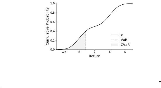
Example 7.18
(Value-at-risk)
.
Let
τ ∈
(0
,
1). The value-at-risk measure (Figure
7.4) corresponds to the τth quantile of the return distribution:
ρ
τ
VaR
(Z) = F
−1
Z
(τ) . 4
7.7 Challenges in Risk-Sensitive Control
Many convenient properties of the risk-neutral objective do not carry over to
risk-sensitive control. As a consequence, finding an optimal policy is usually
significantly more involved. This remains true even when the risk-sensitive
58.
Typically, Problem 7.15 is formulated in terms of a risk to be minimized, which linguistically is
a more natural objective. Here, however, we consider the maximization of
J
ρ
(
π
) so as to keep the
presentation unified with the rest of the book.
Draft version.
Control 215
Figure 7.4
Illustration of value-at-risk (VaR) and conditional value-at-risk (CVaR). Depicted is the
cumulative distribution function of the mixture of normal distributions
ν
=
1
2
N
(0
,
1) +
1
2
N
(4
,
1). The dashed line corresponds to VaR; CVaR (
τ
= 0
.
4) can be determined from
a suitable transformation of the shaded area (see Section 7.8 and Exercise 7.10).
objective (Equation 7.18) can be evaluated efficiently: for example, by using
distributional dynamic programming to approximate the return-distribution func-
tion
η
π
. In this section, we illustrate some of these challenges by characterizing
optimal policies for the variance-constrained control problem.
The variance-constrained problem introduces risk sensitivity by forbidding
policies whose return variance is too high. Given a parameter
C ≥
0, the
objective is to
maximize E
π
[G
π
(X
0
)]
subject to Var
π
G
π
(X
0
)
≤C .
(7.19)
Equation 7.19 can be shown to satisfy our definition of a risk-sensitive control
problem if we express it in terms of a Lagrange multiplier:
J
vc
(π) = min
λ≥0
E
π
G
π
(X
0
)
−λ
Var
π
G
π
(X
0
)
−C
.
The variance-penalized and variance-constrained problems are related in that
they share the Pareto set
π
par
⊆π
h
of possibly optimal solutions. A policy
π
is
in the set π
par
if we have that for all π
0
∈π
h
,
(a) Var
G
π
(X
0
)
> Var
G
π
0
(X
0
)
=⇒ E[G
π
(X
0
)] > E[G
π
0
(X
0
)], and
(b) Var
G
π
(X
0
)
= Var
G
π
0
(X
0
)
=⇒ E[G
π
(X
0
)] ≥E[G
π
0
(X
0
)].
In words, between two policies with equal variances, the one with lower expecta-
tion is never a solution to either problem. However, these problems are generally
not equivalent (Exercise 7.8).
Proposition 7.1 establishes the existence of a solution of the risk-neutral
control problem that is (a) deterministic, (b) stationary, and (c) Markov. By
contrast, the solution to the variance-constrained problem may lack any or all
of these properties.
Draft version.
216 Chapter 7
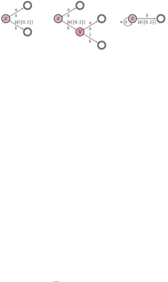
(a) (b) (c)
Figure 7.5
Examples demonstrating how the optimal policy for the variance-constrained control
problem might not be (a) deterministic, (b) Markov, or (c) stationary.
Example 7.19
(The optimal policy may not be deterministic)
.
Consider the
problem of choosing between two actions,
a
and
b
. Action
a
always yields a
reward of 0, while action
b
yields a reward of 0 or 1 with equal probability
(Figure 7.5a). If we seek the policy that maximizes the expected return subject
to the variance constraint
C
=
3
/16
, the best deterministic policy respecting the
variance constraint must choose
a
, for a reward of 0. On the other hand, the
policy that selects
a
and
b
with equal probability achieves an expected reward
of
1
/4 and a variance of
3
/16. 4
Example 7.20
(The optimal policy may not be Markov)
.
Consider the Markov
decision process in Figure 7.5b. Suppose that we seek a policy that maximizes
the expected return from state
x
, now subject to the variance constraint
C
= 0.
Let us assume
γ
= 1 for simplicity. Action
a
has no variance and is therefore
a possible solution, with zero return. Action
b
gives a greater expected return,
at the cost of some variance. Any policy
π
that depends on the state alone
and chooses
b
in state
x
must incur this variance. On the other hand, the
following history-dependent policy achieves a positive expected return without
violating the variance constraint: in state
x
, choose
b
; if the first reward
R
0
is 0,
select action
b
in
x
; otherwise, select action
a
. In all cases, the return is 1, an
improvement over the best Markov policy. 4
Example 7.21
(The optimal policy may not be stationary)
.
In general, the
optimal policy may require keeping track of time. Consider the problem of
maximizing the expected return from the unique state
x
in Figure 7.5c, subject
to
Var
π
(
G
π
(
X
0
))
≤C
, for
C ≤
1
/4
. Exercise 7.9 asks you to show that a simple
time-dependent policy that chooses
a
for
T
C
steps and then selects
b
achieves an
expected return of up to
√
C
. This is possible because the variance of the return
decays at a rate of
γ
2
, while its expected value decays at the slower rate of
γ
.
By contrast, the best randomized stationary policy performs substantially worse
Draft version.
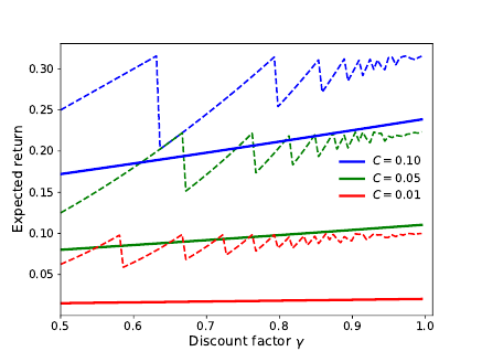
Control 217
Figure 7.6
Expected return as a function of the discount factor
γ
and variance constraint
C
in
Example 7.21. Solid and dashed lines indicate the expected return of the best stationary
and time-dependent policies, respectively. The peculiar zigzag shape of the curve for
the time-varying policy arises because the time
T
C
at which action
b
is taken must be an
integer (see Exercise 7.9).
for a discount factor
γ
close to 1 and small values of
C
(Figure 7.6). Intuitively,
a randomized policy must choose
a
with a sufficiently large probability to avoid
receiving the random reward early, which prevents it from selecting
b
quickly
beyond the threshold of T
C
time steps. 4
The last two examples establish that the variance-constrained risk measure
is time-inconsistent: informally, the agent’s preference for one outcome over
another at time
t
may be reversed at a later time. Compared to the risk-neutral
problem, the variance-constrained problem is more challenging because the
space of policies that one needs to consider is much larger. Among other things,
the lack of an optimal policy that is Markov with respect to the state alone
also implies that the dependency on the initial distribution in Equation 7.19 is
necessary to keep things well defined. The variance-constrained objective must
be optimized for globally, considering the policy at all states at once; this is in
contrast with the risk-neutral setting, where value iteration can make overall
improvements to the policy by acting greedily with respect to the value function
at individual states (see Remark 7.1). In fact, finding an optimal policy for the
variance-constrained control problem is NP-hard (Mannor and Tsitsiklis 2011).
Draft version.

218 Chapter 7
7.8 Conditional Value-At-Risk*
In the previous section, we saw that solutions to the variance-constrained control
problem can take unintuitive forms, including the need to penalize better-than-
expected outcomes. One issue is that variance only coarsely measures what we
mean by “risk” in the common sense of the word. To refine our meaning, we
may identify two types of risk: downside risk, involving undesirable outcomes
such as greater-than-expected losses, and upside risk, involving what we may
informally call a stroke of luck. In some situations, it is possible and useful to
separately account for these two types of risk.
To illustrate this point, we now present a distributional algorithm for optimiz-
ing conditional value-at-risk (CVaR), based on work by Bäuerle and Ott (2011)
and Chow et al. (2015). One benefit of working with full return distributions
is that the algorithmic template we present here can be reasonably adjusted to
deal with other risk measures, including the entropic risk measure described in
Example 7.17. For conciseness, in what follows, we will state without proof a
few technical facts about conditional value-at-risk that can be found in those
sources and the work of Rockafellar and Uryasev (2002).
Conditional value-at-risk measures downside risk by focusing on the lower
tail behavior of the return distribution, specifically the expected value of this
tail. This expected value quantifies the magnitude of losses in extreme scenarios.
Let
Z
be a random variable with cumulative and inverse cumulative distribution
functions
F
Z
and
F
−1
Z
, respectively. For a parameter
τ ∈
(0
,
1), the CVaR of
Z
is
CVaR
τ
(Z) =
1
τ
Z
τ
0
F
−1
Z
(u)du . (7.20)
When the inverse cumulative distribution
F
−1
Z
is strictly increasing, the right-
hand side of Equation 7.20 is equivalent to
E[Z | Z ≤F
−1
Z
(τ)] . (7.21)
In this case, CVaR quantifies the expected return, conditioned on the event that
this return is no greater than the return’s
τ
th quantile – that is, is within the
τ
th
fraction of lowest returns.
59
In a reinforcement learning context, this leads to
the risk-sensitive objective
J
CVaR
(π) = CVaR
τ
∞
X
t=0
γ
t
R
t
. (7.22)
59.
In other fields, CVaR is applied to losses rather than returns, in which case it measures the
expected loss subject that this loss is above the
τ
th percentile. For example, Equation 7.21 becomes
E[Z | Z ≥F
−1
Z
(τ)], and the subsequent derivations need to be adjusted accordingly.
Draft version.
Control 219
In general, there may not be an optimal policy that depends on the state
x
alone;
however, one can show that optimality can be achieved with a deterministic,
stationary Markov policy on an augmented state that incorporates information
about the return thus far. In the context of this section, we assume that rewards
are bounded in [
R
min
, R
max
]. At a high level, we optimize the CVaR objective by
(a) defining the requisite augmented state;
(b)
performing a form of risk-sensitive value iteration on this augmented state,
using a suitable selection rule; and
(c) extracting the resulting policy.
We now explain each of these steps.
Augmented state.
Central to the algorithm and to the state augmentation
procedure is a reformulation of CVaR in terms of a desired minimum return or
target
b ∈R
. Let [
x
]
+
denote the function that is 0 if
x <
0 and
x
otherwise. For
a random variable
Z
and
τ ∈
(0
,
1), Rockafellar and Uryasev (2002) establish
that
CVaR
τ
(Z) = max
b∈R
b −τ
−1
E
[b −Z]
+
. (7.23)
When
F
−1
Z
is strictly increasing, the maximum-achieving
b
for Equation 7.23
is the quantile
F
−1
Z
(
τ
). In fact, taking the derivative of the expression inside
the brackets with respect to
α
yields the quantile update rule (Equation 6.11;
see Exercise 7.11). The advantage of this formulation is that it is more easily
optimized in the context of a policy-dependent return. To see this, let us write
G
π
=
∞
X
t=0
γ
t
R
t
to denote the random return from the initial state
X
0
, following some history-
dependent policy π ∈π
h
. We then have that
max
π∈π
h
J
CVaR
(π) = max
π∈π
h
max
b∈R
b −τ
−1
E
[b −G
π
]
+
= max
b∈R
b −τ
−1
min
π∈π
h
E
[b −G
π
]
+
. (7.24)
In words, the CVaR objective can be optimized by jointly finding an optimal
target
b
and a policy that minimizes the expected shortfall
E
[
b −G
π
]
+
. For a
fixed target
b
, we will see that it is possible to minimize the expected shortfall
by means of dynamic programming. By adjusting
b
appropriately, one then
obtains an optimal policy.
Based on Equation 7.24, let us now consider an augmented state (
X
t
, B
t
),
where
X
t
is as usual the current state and
B
t
takes on values in
B
= [
V
min
, V
max
];
we will describe its dynamics in a moment. With this augmented state, we
Draft version.

220 Chapter 7
may consider a class of stationary Markov policies,
π
CVaR
, which take the form
π : X×B→P(A).
60
We use the variable
B
t
to keep track of the amount of discounted reward
that should be obtained from
X
t
onward in order to achieve a desired minimum
return of
b
0
∈R
over the entire trajectory. The transition structure of the Markov
decision process over the augmented state is defined by modifying the generative
equations (Section 2.3):
B
0
= b
0
A
t
|(X
0:t
, B
0:t
, A
0:t−1
, R
0:t−1
) ∼π(· | X
t
, B
t
)
B
t+1
|(X
0:t+1
, B
0:t
, A
0:t
, R
0:t
) =
B
t
−R
t
γ
;
we similarly extend the sample transition model with the variables
B
and
B
0
.
This definition of the variables (
B
t
)
t≥0
can be understood by noting, for example,
that a minimum return of b
0
is achieved over the whole trajectory if
∞
X
t=1
γ
t−1
R
t
≥
b
0
−R
0
γ
.
If the reward
R
t
is small or negative, the new target
B
t+1
may of course be larger
than
B
t
. Note that the value of
b
0
is a parameter of the algorithm, rather than
given by the environment.
Risk-sensitive value iteration.
We next construct a method for optimizing
the expected shortfall given a target
b
0
∈R
. Let us write
η ∈P
(
R
)
X×B×A
for a
return-distribution function on the augmented state-action space, instantiated
as a return-variable function
G
. For ease of exposition, we will mostly work
with this latter form of the return function. As usual, we write
G
π
for the return-
variable function associated with a policy
π ∈π
CVaR
. With this notation in mind,
we write
J
CVaR
(π, b
0
) = max
b∈R
b −τ
−1
E
[b −G
π
(X
0
, b
0
, A
0
)]
+
(7.25)
to denote the conditional value-at-risk obtained by following policy
π
from the
initial state (X
0
, b
0
), with A
0
∼π(· | X
0
, b
0
).
Similar to distributional value iteration, the algorithm constructs a series of
approximations to the return-distribution function by repeatedly applying the
distributional Bellman operator with a policy derived from a greedy selection
rule
˜
G. Specifically, we write
a
G
(x, b) = arg min
a∈A
E
[b −G(x, b, a)]
+
(7.26)
60. Since B
t
is a function of the trajectory up to time t, π
CVaR
is a strict subset of π
h
.
Draft version.

Control 221
for the greedy action at the augmented state (
x, b
), breaking ties arbitrarily. The
selection rule
˜
G is itself given by
˜
G(η)(a | x, b) =
˜
G(G)(a | x, b) = {a = a
G
(x, b)}.
The algorithm begins by initializing
η
0
(
x, b, a
) =
δ
0
for all
x ∈X
,
b ∈B
, and
a ∈A, and iterating
η
k+1
= T
˜
G
η
k
, (7.27)
as in distributional value iteration. Expressed in terms of return-variable
functions, this is
G
k+1
(x, b, a)
D
= R + γG
k
(X
0
, B
0
, a
G
k
(X
0
, B
0
)), X = x, B = b, A = a.
After
k
iterations, the policy
π
k
=
˜
G
(
η
k
) can be extracted according to Equation
7.26. As suggested by Equation 7.25, a suitable choice of starting state is
b
0
= arg max
b∈B
b −τ
−1
E
[b −G
k
(X
0
, b, a
G
k
(X
0
, b))]
+
. (7.28)
As given, there are two hurdles to producing a tractable implementation of
Equation 7.27: in addition to the usual concern that return distributions may
need to be projected onto a finite-parameter representation, we also have to
contend with a real-valued state variable
B
t
. Before discussing how this can be
addressed, we first establish that Equation 7.27 is a sound approach to finding
an optimal policy for the CVaR objective.
Theorem 7.22.
Consider the sequence of return-distribution functions
(
η
k
)
k≥0
defined by Equation 7.27. Then the greedy policy
π
k
=
˜
G
(
η
k
) is such
that for all x ∈X, b ∈B, and a ∈A,
E
[b −G
π
k
(x, b, a)]
+
≤ min
π∈π
CVaR
E
[b −G
π
(X
0
, b, a)]
+
+
γ
k
V
max
−V
min
1 −γ
.
Consequently, we also have that the conditional value-at-risk of this policy
satisfies (with b
0
given by Equation 7.28)
J
CVaR
(π
k
, b
0
) ≥max
b∈B
max
π∈π
CVaR
J
CVaR
(π, b) −
γ
k
V
max
−V
min
τ(1 −γ)
. 4
The proof is somewhat technical and is provided in Remark 7.3.
Theorem 7.22 establishes that with sufficiently many iterations, the policy
π
k
is close to optimal. Of course, when distribution approximation is intro-
duced, the resulting policy will in general only approximately optimize the
CVaR objective, with an error term that depends on the expressivity of the
probability distribution representation (i.e., the parameter
m
in Chapter 5). To
perform dynamic programming with the state variable
B
, one may use function
Draft version.
222 Chapter 7
approximation, the subject of the next chapter. Another solution is to consider a
discrete number of values for
B
and to extend the operator
T
˜
G
to operate on
this discrete set (Exercise 7.12).
7.9 Technical Remarks
Remark 7.1.
In Section 7.7, we presented some of the challenges involved with
finding an optimal policy for the variance-constrained objective. In some sense,
these challenges should not be too surprising given that that we are looking to
maximize a function
J
of an infinite-dimensional object (a history-dependent
policy). Rather, what should be surprising is the relative ease with which one
can obtain an optimal policy in the risk-neutral setting.
From a technical perspective, this ease is a consequence of Lemma 7.3, which
guarantees that
Q
∗
(and hence
π
∗
) can be efficiently approximated. However,
another important property of the risk-neutral setting is that the policy can be
improved locally: that is, at each state simultaneously. To see this, consider a
state-action value function
Q
π
for a given policy
π
and denote by
π
0
a greedy
policy with respect to Q
π
. Then,
T Q
π
= T
π
0
Q
π
≥T
π
Q
π
= Q
π
. (7.29)
That is, a single step of value iteration applied to the value function of a policy
π
results in a new value function that is at least as good as
Q
π
at all states
– the Bellman operator is said to be monotone. Because this single step also
corresponds to the value of a nonstationary policy that acts according to
π
0
for
one step and then switches to
π
, we can equivalently interpret it as constructing,
one step at a time, a deterministic history-dependent policy for solving the
risk-neutral problem.
By contrast, it is not possible to use a direct dynamic programming approach
over the objective
J
to find the optimal policy for an arbitrary risk-sensitive
control problem. A practical alternative is to perform the optimization instead
with an ascent procedure (e.g., a policy gradient-type algorithm). Ascent algo-
rithms can often be computed in closed form, and tend to be simpler to
implement. On the other hand, convergence is typically only guaranteed to
local optima, seemingly unavoidable when the optimization problem is known
to be computationally hard. 4
Remark 7.2.
When the projection Π
F
is not mean-preserving, distributional
value iteration induces a state-action value function
Q
η
k
that is different from
the value function
Q
k
determined by standard value iteration under equivalent
initial conditions. Under certain conditions on the distributions of rewards, it is
Draft version.

Control 223
possible to bound this difference as
k →∞
. To do so, we use a standard error
bound on approximate value iteration (see, e.g., Bertsekas 2012).
Lemma 7.23. Let (Q
k
)
k≥0
be a sequence of iterates in R
X×A
satisfying
kQ
k+1
−T Q
k
k
∞
≤ε
for some ε > 0 and where T is the Bellman optimality operator. Then,
lim sup
k→∞
kQ
k
−Q
∗
k
∞
≤
ε
1 −γ
. 4
In the context of distributional value iteration, we need to bound the difference
kQ
η
k+1
−T Q
η
k
k
∞
.
When the rewards are bounded on the interval [
R
min
, R
max
] and the projection
step is Π
q
, the
w
1
-projection onto the
m
-quantile representation, a simple bound
follows from an intermediate result used in proving Lemma 5.30 (see Exercise
5.20). In this case, for any ν bounded on [V
min
, V
max
],
w
1
(Π
q
ν, ν) ≤
V
max
−V
min
2m
;
Conveniently, the 1-Wasserstein distance bounds the difference of means
between any distributions ν, ν
0
∈P
1
(R):
E
Z∼ν
[Z] − E
Z∼ν
0
[Z]
≤w
1
(ν, ν
0
) .
This follows from the dual representation of the Wasserstein distance (Villani
2008). Consequently, for any (x, a),
Q
η
k+1
(x, a) −(T
π
k
Q
η
k
)(x, a)
≤w
1
η
k+1
(x, a), (T
π
k
η
k
)(x, a)
= w
1
(Π
q
T
π
k
η
k
)(x, a), (T
π
k
η
k
)(x, a)
≤
V
max
−V
min
2m
.
By taking the maximum over (
x, a
) on the left-hand side of the above and
combining with Lemma 7.23, we obtain
lim sup
k→∞
kQ
η
k
−Q
∗
k
∞
≤
V
max
−V
min
2m(1 −γ)
. 4
Remark 7.3.
Theorem 7.22 is proven from a few facts regarding partial returns,
which we now give. Let us write
a
k
(
x, b
) =
a
G
k
(
x, b
). We define the mapping
U
k
: X×B×A→R as
U
k
(x, b, a) = E
[b −G
k
(x, b, a)]
+
,
and for a policy π ∈π
CVaR
similarly write
U
π
(x, b, a) = E
[b −G
π
(x, b, a)]
+
.
Draft version.
224 Chapter 7
Lemma 7.24. For any x ∈X, a ∈A, b ∈B, and k ∈N, we have
U
k+1
(x, b, a) = γ E
h
U
k
X
0
, B
0
, a
k
(X
0
, B
0
)
| X = x, B = b, A = a
i
.
In addition, if π ∈π
CVaR
is a stationary Markov policy on X×B, we have
U
π
(x, b, a) = γ E
π
h
U
π
X
0
, B
0
, A
0
| X = x, B = b, A = a
i
. 4
Proof.
The result follows by time-homogeneity and the Markov property. Con-
sider the sample transition model (
X, B, A, R, X
0
, B
0
, A
0
), with
A
0
=
a
k
(
X
0
, B
0
).
Simultaneously, consider the partial trajectory (
X
t
, B
t
, A
t
, R
t
)
k
t=0
for which
A
0
= A
0
and A
t
∼π
k−t
(· | X
t
, B
t
) for t > 0. As γB
0
= B −R, we have
γ E
h
U
k
X
0
, B
0
, A
0
| X = x, B = b, A = a
i
= γ E
h
E
h
B
0
−G
k
(X
0
, B
0
, A
0
)
+
i
| X = x, B = b, A = a
i
= γ E
h
E
h
B
0
−
k
X
t=0
γ
t
R
t
+
| X
0
= X
0
, B
0
= B
0
, A
0
= A
0
i
| X = x, A = a
i
= E
h
E
h
b −R −γ
k
X
t=0
γ
t
R
t
+
| X
0
= X
0
, B
0
= B
0
, A
0
= A
0
i
| X = x, B = b, A = a
i
= E
h
E
h
b −R −
k+1
X
t=1
γ
t
R
t
+
| X
1
= X
0
, B
1
= B
0
, A
1
= A
0
i
| X = x, B = b, A = a
i
= E
h
b −
k+1
X
t=0
γ
t
R
t
+
| X
0
= x, B
0
= b, A
0
= a
i
.
The second statement follows similarly. 4
Lemma 7.25.
Suppose that
V
min
≤
0 and
V
max
≥
0. Let (
R
t
)
t≥0
be a sequence of
rewards in [R
min
, R
max
]. For any b ∈R and k ∈N,
E
[b −
∞
X
t=0
γ
t
R
t
]
+
] + γ
k+1
V
min
≤
E
[b −
k
X
t=0
γ
t
R
t
]
+
] ≤E
[b −
∞
X
t=0
γ
t
R
t
]
+
] + γ
k+1
V
max
. 4
Proof. First note that, for any b, z, z
0
∈R,
[b −z]
+
≤[b −z
0
]
+
+ [z
0
−z]
+
. (7.30)
Draft version.

Control 225
To obtain the first inequality in the statement, we set
[b −
∞
X
t=0
γ
t
R
t
]
+
≤[b −
k
X
t=0
γ
t
R
t
]
+
+ [−
∞
X
t=k+1
γ
t
R
t
]
+
.
Since rewards are bounded in [R
min
, R
max
], we have that
−
∞
X
t=k+1
γ
t
R
t
≤−γ
k+1
R
min
1 −γ
= −γ
k+1
V
min
.
As we have assumed that V
min
≤0, it follows that
[b −
∞
X
t=0
γ
t
R
t
]
+
≤[b −
k
X
t=0
γ
t
R
t
]
+
−γ
k+1
V
min
.
The second inequality in the statement is obtained analogously. 4
Lemma 7.26.
The sequence (
η
k
)
k≥0
defined by Equation 7.27 satisfies, for any
x ∈X, b ∈B, and a ∈A,
U
k
(x, b, a) = min
π∈π
CVaR
E
π
[b −
k
X
t=0
γ
t
R
t
]
+
| X = x, B = b, A = a
. (7.31)
4
Proof (sketch).
Our choice of
G
0
(
x, b, a
) = 0 guarantees that the statement is
true for
k
= 0. The result then follows by Lemma 7.24, the fact that the policy
˜
G
(
η
k
) chooses the action minimizing the left-hand side of Equation 7.31, and
by induction on k. 4
Proof of Theorem 7.22.
Let us assume that
V
min
≤
0 and
V
max
≥
0 so that Lemma
7.25 can be applied. This is without loss of generality, as otherwise we may
first construct a new sequence of rewards shifted by an appropriate constant
C
,
such that
R
min
= 0
, R
max
≥
0; by inspection, this transformation does not affect
the statement of the Theorem 7.22.
Let π
∗
∈π
CVaR
be an optimal deterministic policy, in the sense that
U
π
∗
(x, b, a) = min
π∈π
CVaR
U
π
(x, b, a).
Combining Lemmas 7.25 and 7.26, we have
U
π
∗
(x, b, a) + γ
k+1
V
min
≤U
k
(x, b, a) ≤U
π
∗
(x, b, a) + γ
k+1
V
max
. (7.32)
Write E
xba
[·] = E
π
[· | X = x, B = b, A = a]. By Lemma 7.24,
U
π
k
(x, b, a) −U
k
(x, b, a) (7.33)
= γ E
xba
h
U
π
k
(X
0
, B
0
, a
k
(X
0
, B
0
)) −U
k−1
(X
0
, B
0
, a
k−1
(X
0
, B
0
))
i
Draft version.
226 Chapter 7
= γ E
xba
h
U
π
k
(X
0
, B
0
, a
k
(X
0
, B
0
)) −U
k
(X
0
, B
0
, a
k
(X
0
, B
0
))
+ U
k
(X
0
, B
0
, a
k
(X
0
, B
0
)) −U
k−1
(X
0
, B
0
, a
k−1
(X
0
, B
0
))
i
≤γ E
xba
h
U
π
k
(X
0
, B
0
, a
k
(X
0
, B
0
)) −U
k
(X
0
, B
0
, a
k
(X
0
, B
0
))
+ γ
k+1
V
max
−γ
k
V
min
.
Now, the quantity
ε
k
(x, b, a) = U
π
k
(x, b, a) −U
k
(x, b, a)
is bounded above and hence
ε
k
= sup
x∈X,b∈B,a∈A
ε
k
(x, b, a)
exists. Taking the supremum over
x, b
and
a
on both sides of Equation 7.33, we
have
ε
k
≤γε
k
+ γ
k+1
V
max
−γ
k
V
min
and consequently for all x, b, a,
U
π
k
(x, b, a) −U
k
(x, b, a) ≤
γ
k
(γV
max
−V
min
)
1 −γ
. (7.34)
Because U
k
(x, b, a) ≤U
π
∗
(x, b, a) + γ
k+1
V
max
, then
U
π
k
(x, b, a) ≤U
π
∗
(x, b, a) + γ
k+1
V
max
+
γ
k
(γV
max
−V
min
)
1 −γ
.
Now,
γ
k+1
+
γ
k+1
1 −γ
= γ
k
γ + γ(1 −γ)
1 −γ
≤
γ
k
1 −γ
.
Hence, we conclude that also
U
π
k
(x, b, a) ≤ min
π∈π
CVaR
U
π
(x, b, a) +
γ
k
(V
max
−V
min
)
1 −γ
,
as desired.
For the second statement, following Equation 7.28 we have
b
0
= arg max
b∈B
b −τ
−1
E
[b −G
k
(X
0
, b, a
k
(X
0
, b))]
+
.
The algorithm begins in state (
X
0
, b
0
), selects action
A
0
=
a
k
(
X
0
, b
0
), and then
executes policy π
k
from there on; its return is G
π
k
(X
0
, b
0
, A
0
). In particular,
J
CVaR
(π
k
, b
0
) = max
b∈B
b −τ
−1
E
[b −G
π
k
(X
0
, b
0
, A
0
)]
+
≥b
0
−τ
−1
E
[b
0
−G
π
k
(X
0
, b
0
, A
0
)]
+
. (7.35)
Draft version.
Control 227
Write
a
π
∗
(
x, b
) for the action selected by
π
∗
in (
x, b
). Because Equation 7.32
holds for all x, b, and a, we have
min
a∈A
U
k
(x, b, a) ≤min
a∈A
U
π
∗
(x, b, a) + γ
k+1
V
max
=⇒ U
k
(x, b, a
k
(x, b)) ≤U
π
∗
(x, b, a
π
∗
(x, b)) + γ
k+1
V
max
,
since
a
k
(
x, b
) is the action
a
that minimizes
U
k
(
x, b, a
). Hence, for any state
x
,
we have
max
b∈B
b −τ
−1
min
a∈A
U
k
(x, b, a)
≥max
b∈B
b −τ
−1
min
a∈A
U
π
∗
(x, b, a)
−
γ
k+1
V
max
τ
,
and so
b
0
−τ
−1
U
k
(X
0
, b
0
, a
k
(X
0
, b
0
)) ≥max
b∈B
b −τ
−1
U
π
∗
(X
0
, b, a
π
∗
(x, b))
−
γ
k+1
V
max
τ
= max
b∈B
J
CVaR
(π
∗
, b) −
γ
k+1
V
max
τ
.
Combined with Equations 7.34 and 7.35, this yields
J
CVaR
(π
k
, b
0
) ≥max
b∈B
max
π∈π
CVaR
J
CVaR
(π, b) −
γ
k
(V
max
−V
min
)
τ(1 −γ)
. 4
7.10 Bibliographical Remarks
7.0.
The balloon navigation example at the beginning of the chapter is from
Bellemare et al. (2020). Sutton and Barto (2018) separate “control problem”
from “prediction problem”; the latter figures more predominantly in this book.
In earlier literature, the control problem comes first (see, e.g., Bellman 1957b)
and prediction is typically used as a subroutine for control (Howard 1960).
7.1.
Time-dependent policies are common in finite-horizon scenarios and are
studied at length by Puterman (2014). The technical core of Proposition 7.2
involves demonstrating that any feasible value function can be attained by a
stationary Markov policy; see the results by Puterman (2014, Theorem 5.5.1),
Altman (1999) and the discussion by Szepesvári (2020).
In reinforcement learning, history-dependent policies are also used to deal
with partially observable environments, in which the agent receives an obser-
vation
o
at each time step rather than the identity of its state. For example,
McCallum (1995) uses a variable-length history to represent state-action values,
while Veness et al. (2011) use a history-based probabilistic model to learn a
model of the environment. History-dependent policies also play a central role
in the study of optimality in the fairly large class of computable environments
(Hutter 2005).
Draft version.
228 Chapter 7
7.2.
The canonical reference for value iteration is the book by Bellman (1957b);
see also Bellman (1957a) for an asymptotic analysis in the undiscounted set-
ting. Lemma 7.3 is standard and can be found in most reinforcement learning
textbooks (Bertsekas and Tsitsiklis 1996; Szepesvári 2010; Puterman 2014).
State-action value functions were introduced along with the Q-learning algo-
rithm (Watkins 1989) and subsequently used in the development of SARSA
(Rummery and Niranjan 1994). Watkins and Dayan (1992) give a restricted
result regarding the convergence of Q-learning, which is more thoroughly estab-
lished by Jaakkola et al. (1994), Tsitsiklis (1994), and Bertsekas and Tsitsiklis
(1996).
7.3–7.5.
The expression of the optimality operator as a fixed-policy operator
whose policy varies with the input is common in the analysis of control algo-
rithms (see, e.g., Munos 2003; Scherrer 2014). The view of value iteration as
constructing a history-dependent policy is taken by Scherrer and Lesner (2012)
to derive more accurate value learning algorithms in the approximate setting.
The extension to distributional value iteration and Theorem 7.13 are from
Bellemare et al. (2017a). The correspondence between standard value iteration
and distributional value iteration with a mean-preserving projection is given by
Lyle et al. (2019).
The notion of action gap plays an important role in understanding the rela-
tionship between value function estimates and policies, in particular when
estimates are approximate. Farahmand (2011) gives a gap-dependent bound on
the expected return obtained by a policy derived from an approximate value
function. Bellemare et al. (2016) derive an algorithm for increasing the action
gap so as to improve performance in the approximate setting.
An example of a selection rule that explicitly incorporates distributional
information is the lexicographical rule of Jaquette (1973), which orders policies
according to the magnitude of their moments.
7.6.
The notion of risk and risk-sensitive decisions can be traced back to
Markowitz (1952), who introduced the concept of trading off expected gains and
variations in those gains in the context of constructing an investment portfolio;
see also Steinbach (2001) for a retrospective. Artzner et al. (1999) propose a
collection of desirable characteristics that make a risk measure coherent in the
sense that it satisfies certain preference axioms. Of the risk measures mentioned
here, CVaR is coherent but the variance-constrained objective is not. Artzner et
al. (2007) discuss coherent risk measures in the context of sequential decisions.
Ruszczy
´
nski (2010) introduces the notion of dynamic risk measures for Markov
decision processes, which are amenable to optimization via Bellman-style recur-
sions; see also Chow (2017) for a discussion of static and dynamic risk measures
Draft version.
Control 229
as well as time consistency. Jiang and Powell (2018) develop sample-based
optimization methods for dynamic risk measures based on quantiles.
Howard and Matheson (1972) considered the optimization of an exponential
utility function applied to the random return by means of policy iteration. The
same objective is given a distributional treatment by Chung and Sobel (1987).
Heger (1994) considers optimizing for worst-case returns. Haskell and Jain
(2015) study the use of occupancy measures over augmented state spaces as an
approach for finding optimal policies for risk-sensitive control; similarly, an
occupancy measure-based approach to CVaR optimization is studied by Carpin
et al. (2016). Mihatsch and Neuneier (2002) and Shen et al. (2013) extend
Q-learning to the optimization of recursive risk measures, where a base risk
measure is applied at each time step. Recursive risk measures are more easily
optimized than risk measures directly applied to the random return but are not
as easily interpreted. Martin et al. (2020) consider combining distributional
reinforcement learning with the notion of second-order stochastic dominance as
a means of action selection. Quantile criteria are considered by Filar et al. (1995)
in the case of average-reward MDPs and, more recently, by Gilbert et al. (2017)
and Li et al. (2022). Delage and Mannor (2010) solve a risk-constrained opti-
mization problem to handle uncertainty in a learned model’s parameters. See
Prashanth and Fu (2021) for a survey on risk-sensitive reinforcement learning.
7.7.
Sobel (1982) establishes that an operator constructed directly from the
variance-penalized objective does not have the monotone improvement prop-
erty, making its optimization more challenging. The examples demonstrating
the need for randomization and a history-dependent policy are adapted from
Mannor and Tsitsiklis (2011), who also prove the NP-hardness of the problem
of optimizing the variance-constrained objective. Tamar et al. (2012) propose
a policy gradient algorithm for optimizing a mean-variance objective and for
the CVaR objective (Tamar et al. 2015); see also Prashanth and Ghavamzadeh
(2013) and Chow and Ghavamzadeh (2014) for actor-critic algorithms for these
criteria. Chow et al. (2018) augment the state with the return-so-far in order to
extend gradient-based algorithms to a broader class of risk measures.
7.8.
The reformulation of the conditional value-at-risk (CVaR) of a random
variable in terms of the (convex) optimization of a function of a variable b ∈R
is due to Rockafellar and Uryasev (2000); see also Rockafellar and Uryasev
(2002) and Shapiro et al. (2009). Bäuerle and Ott (2011) provide an algorithm
for optimizing the CVaR of the random return in Markov decision processes.
Their work forms the basis for the algorithm presented in this section, although
the treatment in terms of return-distribution functions is new here. Another
closely related algorithm is due to Chow et al. (2015), who additionally provide
an approximation error bound on the computed CVaR. Brown et al. (2020) apply
Draft version.
230 Chapter 7
Rockafellar and Uryasev’s approach to design an agent that is risk-sensitive
with respect to a prior distribution over possible reward functions. Keramati et
al. (2020) combine categorical temporal-difference learning with an exploration
bonus derived from the Dvoretzky–Kiefer–Wolfowitz inequality to develop an
algorithm to optimize for conditional value-at-risk.
7.11 Exercises
Exercise 7.1.
Find a counterexample that shows that the Bellman optimality
operator is not an affine operator. 4
Exercise 7.2.
Consider the Markov decision process depicted in Figure 2.4a.
For which values of the discount factor
γ ∈
[0
,
1) is there more than one optimal
action from state
x
? Use this result to argue that the optimal policy depends on
the discount factor. 4
Exercise 7.3.
Proposition 7.7 establishes that distributional Bellman optimality
operators are not contraction mappings.
(i)
Instantiate the result with the 1-Wasserstein distance. Provide a visual
explanation for the result by drawing the relevant cumulative distribution
functions before and after the application of the operator.
(ii)
Discuss why it was necessary, in the proof of Proposition 7.7, to assume
that the probability metric d is c-homogeneous. 4
Exercise 7.4.
Suppose that there is a unique optimal policy
π
∗
, as per Section
7.4. Consider the use of a projection Π
F
for a probability representation
F
and
the iterates
η
k+1
= Π
F
Tη
k
. (7.36)
Discuss under what conditions the sequence of greedy policies (
G
(
η
k
))
k≥0
converges to π
∗
when Π
F
is
(i) the m-categorical projection Π
c
;
(ii) the m-quantile projection Π
q
.
Where necessary, provide proofs of your statements. Does your answer depend
on m or on θ
1
, . . . , θ
m
for the case of the categorical representation? 4
Exercise 7.5.
Give a Markov decision process for which the limit of the
sequence of iterates defined by
η
k+1
=
T
G
η
k
depends on the initial condition
η
0
,
irrespective of the greedy selection rule
G
. Hint. Construct a scenario where the
implied policy π
k
is the same for all k but depends on η
0
. 4
Exercise 7.6.
Consider the greedy selection rule that selects an action with
minimal variance among those with maximal expected value, breaking ties
Draft version.

Control 231
uniformly at random. Provide an example Markov decision process in which
this rule results in a sequence of return-distribution functions that does not
converge, as per Example 7.11. Hint. Consider reward distributions of the form
1
3
P
3
i=1
δ
θ
i
. 4
Exercise 7.7
(*)
.
Consider the 1-Wasserstein distance
w
1
and its supremum
extension
w
1
. In addition, let
d
be a metric on
P
(
A
). Suppose that we are given
a mapping
˜
G: P(R)
X×A
→π
ms
which is continuous at every state, in the sense that for any
ε >
0, there exists a
δ > 0 such that for any return functions η, η
0
,
w
1
(η, η
0
) < δ =⇒ max
x∈X
d
˜
G(η)(· | x),
˜
G(η
0
)(· | x)
< ε.
Show that this mapping cannot be a greedy selection rule in the sense of
Definition 7.6. 4
Exercise 7.8.
Consider the Markov decision process depicted in Figure 7.5a.
Show that there is no λ ≥0 such that the policy maximizing
J
mv
(π) = E
π
G
π
(X
0
)
−λVar
π
G
π
(X
0
)
is stochastic. This illustrates how the variance-constrained and variance-
penalized control problems are not equivalent. 4
Exercise 7.9. Consider the Markov decision process depicted in Figure 7.5c.
(i)
Solve for the optimal stopping time
T
C
maximizing the return of a time-
dependent policy that selects action
a
for
T
C
time steps, then selects action
b (under the constraint that the variance should be no greater than C).
(ii) Prove that this policy can achieve an expected return of up to
√
C.
(iii) Based on your conclusions, design a policy that improves on this strategy.
(iv)
Show that the expectation and variance of the return of a randomized
stationary policy that selects action b with probability p are given by
E
π
[G
π
(x)] =
p
2
1 −γ(1 − p)
Var
π
G
π
(x)
=
p
4
2
1 −γ
2
(1 − p)
−
p
(1 −γ(1 − p))
2
!
.
(v)
Using your favorite visualization program, chart the returns achieved by the
optimal randomized policy and the optimal time-dependent policy, for values
of
C
and
γ
different from those shown in Figure 7.5c. What do you observe?
Hint. Use a root-finding algorithm to determine the maximum expected
return of a randomized policy under the constraint Var
π
G
π
(x)
≤C. 4
Draft version.

232 Chapter 7
Exercise 7.10.
Explain the relationship between the shaded area in Figure 7.4
and conditional value-at-risk for the depicted distribution. 4
Exercise 7.11.
Following Equation 7.23, for a distribution
ν ∈P
(
R
), consider
the function
f (θ) = θ −τ
−1
E
Z∼ν
[θ −Z]
+
.
Show that for τ ∈(0, 1),
θ ←θ −ατ
d
dθ
f (θ)
is equivalent to the quantile update rule (Equation 6.11), in expectation. 4
Exercise 7.12
(*)
.
Consider a uniform discretization
B
ε
of the interval
[
V
min
, V
max
] into intervals of width
ε
(endpoints included). For a return-
distribution function
η
on the discrete space
X×B
ε
×A
, define its extension to
X×[V
min
, V
max
] ×A
˜η(x, b, a) = η(x, ε
j
b
ε
k
, a).
Suppose that probability distributions can be represented exactly (i.e., without
needing to resort to a finite-parameter representation). For the CVaR objective
(Equation 7.22), derive an upper bound for the suboptimality
max
π∈π
CVaR
J(π) − J( ˜π),
where
˜π
is found by the procedure of Section 7.8 applied to the discrete space
X×B
ε
×A and using the extension η 7→ ˜η to implement the operator T
˜
G
. 4
Draft version.