6
Incremental Algorithms
The concept of experience is central to reinforcement learning. Methods such
as TD and categorical TD learning iteratively update predictions on the basis of
transitions experienced by interacting with an environment. Such incremental
algorithms are applicable in a wide range of scenarios, including those in
which no model of the environment is known, or in which the model is too
complex to allow for dynamic programming methods to be applied. Incremental
algorithms are also often easier to implement. For these reasons, they are key in
the application of reinforcement learning to many real-world domains.
With this ease of use, however, comes an added complication. In contrast to
dynamic programming algorithms, which steadily make progress toward the
desired goal, there is no guarantee that incremental methods will generate con-
sistently improving estimates of return distributions from iteration to iteration.
For example, an unusually high reward in a sampled transition may actually
lead to a short-term degrading of the value estimate for the corresponding state.
In practice, this requires making sufficiently small steps with each update, to
average out such variations. In theory, the stochastic nature of incremental
updates makes the analysis substantially more complicated than contraction
mapping arguments.
This chapter takes a closer look at the behavior and design of incremen-
tal algorithms – distributional and not. Using the language of operators and
probability distribution representations, we also formalize what it means for an
incremental algorithm to perform well and discuss how to analyze its asymptotic
convergence to the desired estimate.
6.1 Computation and Statistical Estimation
Iterative policy evaluation finds an approximation to the value function
V
π
by
successively computing the iterates
V
k+1
= T
π
V
k
, (6.1)
Draft version. 161
162 Chapter 6
defined by an arbitrary initial value function estimate
V
0
∈R
X
. We can also
think of temporal-difference learning as computing an approximation to the
value function
V
π
, albeit with a different mode of operation. To begin, recall
from Chapter 3 the TD learning update rule:
V(x) ←(1 −α)V(x) + α
r + γV(x
0
)
. (6.2)
One of the aims of this chapter is to study the long-term behavior of the value
function estimate
V
(and, eventually, of estimates produced by incremental,
distributional algorithms).
At the heart of our analysis is the behavior of a single update. That is, for a
fixed
V ∈R
X
, we may understand the learning dynamics of temporal-difference
learning by considering the random value function estimate
V
0
defined via the
sample transition model (X = x, A, R, X
0
):
V
0
(x) = (1 −α)V(x) + α
R + γV(X
0
)
, (6.3)
V
0
(y) = V(y) , y , x .
There is a close connection between the expected effect of the update given by
Equation 6.3 and iterative policy evaluation. Specifically, the expected value of
the quantity
R
+
γV
(
X
0
) precisely corresponds to the application of the Bellman
operator to V, evaluated at the source state x:
E
π
[R + γV(X
0
) | X = x] = (T
π
V)(x) .
Consequently, in expectation TD learning adjusts its value function estimate at
x in the direction given by the Bellman operator:
E
π
[V
0
(x) | X = x] = (1 −α)V(x) + α(T
π
V)(x) . (6.4)
To argue that temporal-difference learning correctly finds an approximation to
V
π
, we must also be able to account for the random nature of TD updates. An
effective approach is to rewrite Equation 6.3 as the sum of an expected target
and a mean-zero noise term:
V
0
(x) = (1 −α)V(x) + α
(T
π
V)(x)
| {z }
expected target
+ R + γV(X
0
) −(T
π
V)(x)
| {z }
noise
; (6.5)
with this decomposition, we may simultaneously analyze the mean dynamics of
TD learning as well as the effect of the noise on the value function estimates. In
the second half of the chapter, we will use Equation 6.5 to establish that under
appropriate conditions, these dynamics can be controlled so as to guarantee
the convergence of temporal-difference learning to
V
π
and analogously the
convergence of categorical temporal-difference learning to the fixed point ˆη
π
c
.
Draft version.
Incremental Algorithms 163
6.2 From Operators to Incremental Algorithms
As illustrated in the preceding section, we can explain the behavior of temporal-
difference learning (an incremental algorithm) by relating it to the Bellman
operator. New incremental algorithms can also be obtained by following the
reverse process – by deriving an update rule from a given operator. This tech-
nique is particularly effective in distributional reinforcement learning, where
one often needs to implement incremental counterparts to a variety of dynamic
programming algorithms. To describe how one might derive an update rule
from an operator, we now introduce an abstract framework based on what is
known as stochastic approximation theory.
45
Let us assume that we are given a contractive operator
O
over some state-
indexed quantity and that we are interested in determining the fixed point
U
∗
of
this operator. With dynamic programming methods, we obtain an approximation
of U
∗
by computing the iterates
U
k+1
(x) = (OU
k
)(x) , for all x ∈X.
To construct a corresponding incremental algorithm, we must first identify what
information is available at each update; this constitutes our sampling model.
For example, in the case of temporal-difference learning, this is the sample
transition model (
X, A, R, X
0
). For Monte Carlo algorithms, the sampling model
is the random trajectory (
X
t
, A
t
, R
t
)
t≥0
(see Exercise 6.1). In the context of this
chapter, we assume that the sampling model takes the form (
X, Y
), where
X
is
the source state to be updated, and
Y
comprises all other information in the
model, which we term the sample experience.
Given a step size
α
and realizations
x
and
y
of the source state variable
X
and
sample experience
Y
, respectively, we consider incremental algorithms whose
update rule can be expressed as
U(x) ←(1 −α)U(x) + α
ˆ
O(U, x, y) . (6.6)
Here,
ˆ
O
(
U, x, y
) is a sample target that may depend on the current estimate
U
. Typically, the particular setting we are in also imposes some limitation on
the form of
ˆ
O
. For example, when
O
is the Bellman operator
T
π
, although
ˆ
O
(
U, x, y
) = (
OU
)(
x
) is a valid instantiation of Equation 6.6, its implementation
might require knowledge of the environment’s transition kernel and reward
function. Implicit within Equation 6.6 is the notion that the space that the
estimate
U
occupies supports a mixing operation; this will indeed be the case
45.
Our treatment of incremental algorithms and their relation to stochastic approximation theory is
far from exhaustive; the interested reader is invited to consult the bibliographical remarks.
Draft version.

164 Chapter 6
for the algorithms we consider in this chapter, which work either with finite-
dimensional parameter sets or probability distributions themselves.
With this framework in mind, the question is what makes a sensible choice
for
ˆ
O.
Unbiased update.
An important case is when the sample target
ˆ
O
can be
chosen so that in expectation, it corresponds to the application of the operator
O:
E[
ˆ
O(U, X, Y) | X = x] = (OU)(x) . (6.7)
In general, when Equation 6.7 holds, the resulting incremental algorithm is
also well behaved. More formally, we will see that under reasonable conditions,
the estimates produced by such an algorithm are guaranteed to converge to
U
∗
– a generalization of our earlier statement that temporal-difference learning
converges to V
π
.
Conversely, when the operator
O
can be expressed as an expectation over
some function of
U
,
X
, and
Y
, then it is possible to derive a sample target simply
by substituting the random variables involved with their realizations. In effect,
we then use the sample experience to construct an unbiased estimate of (
OU
)(
x
).
As a concrete example, the TD target, expressed in terms of random variables,
is
ˆ
O(V, X, Y) = R + γV(X
0
) ;
the corresponding update rule is
V(x) ←(1 −α)V(x) + α (r + γV(x
0
))
| {z }
sample target
.
In the next section, we will show how to use this approach to derive categorical
temporal-difference learning (introduced in Chapter 3) from the categorical-
projected Bellman operator.
Example 6.1.
The consistent Bellman operator is an operator over state-action
value functions based on the idea of making consistent choices at each state. At
a high level, the consistent operator adds the constraint that actions that leave
the state unchanged should be repeated. This operator is formalized as
T
π
c
Q(x, a) = E
π
R + γ max
a
0
∈A
Q(X
0
, a
0
)
{X
0
, x}
+ γQ(x, a)
{X
0
= x}
| X = x
.
Let (
x, a, r, x
0
) be drawn according to the sample transition model. The update
rule derived by substitution is
Q(x, a) ←
(1 −α)Q(x, a) + α
r + γ max
a
0
∈A
Q(x
0
, a
0
)
if x
0
, x
(1 −α)Q(x, a) + α(r + γQ(x, a)) otherwise.
Draft version.
Incremental Algorithms 165
Compared to Q-learning (Section 3.7), the consistent update rule increases the
action gap at each state, in the sense that its operator’s fixed point
Q
∗
c
has the
property that for all (x, a) ∈X×A,
max
a
0
∈A
Q
∗
c
(x, a
0
) −Q
∗
c
(x, a) ≥max
a
0
∈A
Q
∗
(x, a
0
) −Q
∗
(x, a) ,
with strict inequality whenever P
X
(x | x, a) > 0. 4
A general principle.
Sometimes, expressing the operator
O
in the form of
Equation 6.7 requires information that is not available to our sampling model.
In this case, it is sometimes still possible to construct an update rule whose
repeated application approximates the operator
O
. More precisely, given a fixed
estimate
˜
U
, with this approach we look for a sample target function
ˆ
O
such that
from a suitable initial condition, repeated updates of the form
U(x) ←(1 −α)U(x) + α
ˆ
O(
˜
U, x, y)
lead to
U ≈O
˜
U
. In this case, a necessary condition for
ˆ
O
to be a suitable sample
target is that it should leave the fixed point U
∗
unchanged, in expectation:
E
π
[
ˆ
O(U
∗
, X, Y) | X = x] = U
∗
(x) .
In Section 6.4, we will introduce quantile temporal-difference learning, an
algorithm that applies this principle to find the fixed point of the quantile-
projected Bellman operator.
6.3 Categorical Temporal-Difference Learning
Categorical dynamic programming (CDP) computes a sequence (
η
k
)
k≥0
of
return-distribution functions, defined by iteratively applying the projected dis-
tributional Bellman operator Π
c
T
π
to an initial return-distribution function
η
0
:
η
k+1
= Π
c
T
π
η
k
.
As we established in Section 5.9, the sequence generated by CDP converges
to the fixed point
ˆη
π
c
. Let us express this fixed point in terms of a collection of
probabilities
(
p
π
i
(
x
))
m
i=1
:
x ∈X
associated with
m
particles located at
θ
1
, . . . , θ
m
:
ˆη
π
c
(x) =
m
X
i=1
p
π
i
(x)δ
θ
i
.
To derive an incremental algorithm from the categorical-projection Bellman
operator, let us begin by expressing the projected distributional operator Π
c
T
π
in terms of an expectation over the sample transition (X = x, A, R, X
0
):
Π
c
T
π
η
(x) = Π
c
E
π
h
b
R,γ
#
η
π
(X
0
) | X = x
i
. (6.8)
Draft version.

166 Chapter 6
Following the line of reasoning from Section 6.2, in order to construct an
unbiased sample target by substituting
R
and
X
0
with their realizations, we
need to rewrite Equation 6.8 with the expectation outside of the projection Π
c
.
The following establishes the validity of exchanging the order of these two
operations.
Proposition 6.2.
Let
η ∈F
X
C,m
be a return function based on the
m
-
categorical representation. Then for each state x ∈X,
(Π
c
T
π
η
(x) = E
π
Π
c
(b
R,γ
)
#
η(X
0
)
| X = x
. 4
Proposition 6.2 establishes that the projected operator Π
c
T
π
can be written
in such a way that the substitution of random variables with their realizations
can be performed. Consequently, we deduce that the random sample target
ˆ
O
η, x, (R, X
0
)
= Π
c
(b
R,γ
)
#
η(X
0
)
provides an unbiased estimate of (Π
c
T
π
η
)(
x
). For a given realization (
x, a, r, x
0
)
of the sample transition, this leads to the update rule
46
η(x) ←(1 −α)η(x) + αΠ
c
(b
r,γ
)
#
η(x
0
)
| {z }
sample target
. (6.9)
The last part of the CTD derivation is to express Equation 6.9 in terms of
the actual parameters being updated. These parameters are the probabilities
(p
i
(x))
m
i=1
: x ∈X
of the return-distribution function estimate η:
η(x) =
m
X
i=1
p
i
(x)δ
θ
i
.
The sample target in Equation 6.9 is given by the pushforward transformation of
a
m
-categorical distribution (
η
(
x
0
)) followed by a categorical projection. As we
demonstrated in Section 3.6, the projection of a such a transformed distribution
can be expressed concisely from a set of coefficients (
ζ
i, j
(
r
) :
i, j ∈{
1
, . . . , m}
).
In terms of the triangular and half-triangular kernels (
h
i
)
m
i=1
that define the
categorical projection (Section 5.6), these coefficients are
ζ
i, j
(r) = h
i
ς
−1
m
(r + γθ
j
−θ
i
)
. (6.10)
With these coefficients, the update rule over the probability parameters is
p
i
(x) ←(1 −α)p
i
(x) + α
m
X
j=1
ζ
i, j
(r)p
j
(x
0
) .
46.
Although the action
a
is not needed to construct the sample target, we include it for consistency.
Draft version.

Incremental Algorithms 167
Our derivation illustrates how substituting random variables for their real-
izations directly leads to an incremental algorithm, provided we have the right
operator to begin with. In many situations, this is simpler than the step-by-
step process that we originally followed in Chapter 3. Because the random
sample target is an unbiased estimate of the projected Bellman operator, it
is also simpler to prove its convergence to the fixed point
ˆη
π
c
; in the second
half of this chapter, we will in fact apply the same technique to analyze both
temporal-difference learning and CTD.
Proof of Proposition 6.2. For a given r ∈R, x
0
∈X, let us write
˜η(r, x
0
) = (b
r,γ
)
#
η(x
0
) .
Fix x ∈X. For conciseness, let us define, for z ∈R,
˜
h
i
(z) = h
i
ς
−1
m
(z −θ
i
)
.
With this notation, we have
E
π
Π
c
(b
R,γ
)
#
η(X
0
)
| X = x
(a)
= E
π
h
m
X
i=1
δ
θ
i
E
Z∼˜η(R,X
0
)
[
˜
h
i
(Z)] | X = x
i
=
m
X
i=1
δ
θ
i
E
π
h
E
Z∼˜η(R,X
0
)
[
˜
h
i
(Z)] | X = x
i
(b)
=
m
X
i=1
δ
θ
i
E
Z
0
∼(T
π
η)(x)
˜
h
i
(Z
0
)
= Π
c
(T
π
η)(x) ,
where (a) follows by definition of the categorical projection in terms of the
triangular and half-triangular kernels (
h
i
)
m
i=1
and (b) follows by noting that
if the conditional distribution of
R
+
γG
(
X
0
) (where
G
is an instantiation of
η
independent of the sample transition (
x, A, R, X
0
)) given
R, X
0
is
˜η
(
R, X
0
) =
(
b
R,γ
)
#
η
(
X
0
), then the unconditional distribution of
G
when
X
=
x
is (
T
π
η
)(
x
).
6.4 Quantile Temporal-Difference Learning
Quantile regression is a method for determining the quantiles of a probability
distribution incrementally and from samples.
47
In this section, we develop an
47.
More precisely, quantile regression is the problem of estimating a predetermined set of quantiles
of a collection of probability distributions. By extension, in this book, we also use “quantile
regression” to refer to the incremental method that solves this problem.
Draft version.
168 Chapter 6
algorithm that aims to find the fixed point
ˆη
π
q
of the quantile-projected Bellman
operator Π
q
T
π
via quantile regression.
To begin, suppose that given
τ ∈
(0
,
1), we are interested in estimating the
τ
th quantile of a distribution
ν
, corresponding to
F
−1
ν
(
τ
). Quantile regression
maintains an estimate
θ
of this quantile. Given a sample
z
drawn from
ν
, it
adjusts θ according to
θ ←θ + α(τ −
{z < θ}
) . (6.11)
One can show that quantile regression follows the negative gradient of the
quantile loss
48
L
τ
(θ) = (τ −
{z < θ}
)(z −θ)
= |
{z < θ}
−τ|×|z −θ|. (6.12)
In Equation 6.12, the term
|
{z < θ}
−τ|
is an asymmetric step size that is either
τ
or 1
−τ
, according to whether the sample
z
is greater or smaller than
θ
,
respectively. When
τ <
0
.
5, samples greater than
θ
have a lesser effect on it
than samples smaller than
θ
; the effect is reversed when
τ >
0
.
5. The update
rule in Equation 6.11 will continue to adjust the estimate until the equilibrium
point
θ
∗
is reached (Exercise 6.4 asks you to visualize the behavior of quantile
regression with different distributions). This equilibrium point is the location at
which smaller and larger samples have an equal effect in expectation. At that
point, letting Z ∼ν, we have
0 = E
τ −
{Z < θ
∗
}
= τ −E
{Z < θ
∗
}
= τ −P(Z < θ
∗
)
=⇒ P(Z < θ
∗
) = τ
=⇒ θ
∗
= F
−1
ν
(τ) . (6.13)
For ease of exposition, in the final line we assumed that there is a unique
z ∈R
for which F
ν
(z) = τ; Remark 6.1 discusses the general case.
Now, let us consider applying quantile regression to find a
m
-quantile approx-
imation to the return-distribution function (ideally, the fixed point
ˆη
π
q
). Recall
that a
m
-quantile return-distribution function
η ∈F
X
Q,m
is parameterized by the
locations
(θ
i
(x))
m
i=1
: x ∈X
:
η(x) =
1
m
m
X
i=1
δ
θ
i
(x)
.
48.
More precisely, Equation 6.11 updates
θ
in the direction of the negative gradient of
L
τ
provided
that P
Z∼ν
(Z = θ) = 0. This holds trivially if ν is a continuous probability distribution.
Draft version.
Incremental Algorithms 169
Now, the quantile projection Π
q
ν of a probability distribution ν is given by
Π
q
ν =
1
m
m
X
i=1
δ
F
−1
ν
(τ
i
)
, τ
i
=
2i −1
2m
for i = 1, …, m .
Given a source state
x ∈X
, the general idea is to perform quantile regression for
all location parameters (
θ
i
)
m
i=1
simultaneously, using the quantile levels (
τ
i
)
m
i=1
and samples drawn from (
T
π
η
)(
x
). To this end, let us momentarily introduce a
random variable
J
uniformly distributed on
{
1
, . . . , m}
. By Proposition 4.11, we
have
D
π
R + γθ
J
(X
0
) | X = x
= (T
π
η)(x) . (6.14)
Given a realized transition (
x, a, r, x
0
), we may therefore construct
m
sample
targets
r
+
γθ
j
(
x
0
)
m
j=1
. Applying Equation 6.11 to these targets leads to the
update rule
θ
i
(x) ←θ
i
(x) +
α
m
m
X
j=1
τ
i
− {r + γθ
j
(x
0
) < θ
i
(x)}
, i = 1, . . . m . (6.15)
This is the quantile temporal-difference learning (QTD) algorithm. A concrete
instantiation in the online case is summarized by Algorithm 6.1, by analogy with
the presentation of categorical temporal-difference learning in Algorithm 3.4.
Note that applying Equation 6.15 requires computing a total of
m
2
terms per
location; when
m
is large, an alternative is to instead use a single term from
the sum in Equation 6.15, with
j
sampled uniformly at random. Interestingly
enough, for
m
sufficiently small, the per-step cost of QTD is less than the cost
of sorting the full distribution (
T
π
η
)(
x
) (which has up to
N
X
N
R
m
particles).
This suggests that the quantile regression approach to the projection step may
be useful even in the context of distributional dynamic programming.
The use of quantile regression to derive QTD can be seen as an instance of
the principle introduced at the end of Section 6.2. Suppose that we consider an
initial return function
η
0
(x) =
1
m
m
X
j=1
δ
θ
0
j
(x)
.
If we substitute the sample target in Equation 6.15 by a target constructed from
this initial return function, we obtain the update rule
θ
i
(x) ←θ
i
(x) +
α
m
m
X
j=1
τ
i
− {r + γθ
0
j
(x
0
) < θ
i
(x)}
, i = 1, . . . m . (6.16)
By inspection, we see that Equation 6.16 corresponds to quantile regression
applied to the problem of determining, for each state
x ∈X
, the quantiles of
Draft version.

170 Chapter 6
Algorithm 6.1: Online quantile temporal-difference learning
Algorithm parameters: step size α ∈(0, 1],
policy π : X→P(A),
number of quantiles m,
initial locations
(θ
0
i
(x))
m
i=1
: x ∈X
θ
i
(x) ←θ
0
i
(x) for i = 1, . . . , m, x ∈X
τ
i
←
2i−1
2m
for i = 1, . . . , m
Loop for each episode:
Observe initial state x
0
Loop for t = 0, 1, . . .
Draw a
t
from π(· | x
t
)
Take action a
t
, observe r
t
, x
t+1
for i = 1, …, m do
θ
0
i
←θ
i
(x
t
)
for j = 1, …, m do
if x
t+1
is terminal then
g ←r
t
else
g ←r
t
+ γθ
j
(x
t+1
)
θ
0
i
←θ
0
i
+
α
m
τ
i
− {g < θ
i
(x
t
)}
end for
end for
for i = 1, …, m do
θ
i
(x
t
) ←θ
0
i
end for
until x
t+1
is terminal
end
the distribution (
T
π
η
0
)(
x
). Consequently, one may think of quantile temporal-
difference learning as performing an update that would converge to the quantiles
of the target distribution, if that distribution were held fixed.
Based on this observation, we can verify that QTD is a reasonable distribu-
tional reinforcement learning algorithm by considering its behavior at the fixed
point
ˆη
π
q
= Π
q
T
π
ˆη
π
q
,
the solution found by quantile dynamic programming. Let us denote the param-
eters of this return function by
ˆ
θ
π
i
(
x
), for
i
= 1
, . . . , m
and
x ∈X
. For a given
Draft version.

Incremental Algorithms 171
state x, consider the intermediate target
˜η(x) =
T
π
ˆη
π
q
(x) .
Now, by definition of the quantile projection operator, we have
ˆ
θ
π
i
(x) = F
−1
˜η(x)
2i−1
2m
.
However, by Equation 6.13, we also know that the quantile regression update
rule applied at
ˆ
θ
π
i
(
x
) with
τ
i
=
2i−1
2m
leaves the parameter unchanged in expec-
tation. In other words, the collection of locations
ˆ
θ
π
i
(
x
)
m
i=1
is a fixed point of
the expected quantile regression update, and consequently the return function
ˆη
π
q
is a solution of the quantile temporal-difference learning algorithm. This
gives some intuition that is it indeed a valid learning rule for distributional
reinforcement learning with quantile representations.
Before concluding, it is useful to illustrate why the straightforward approach
taken to derive categorical temporal-difference learning, based on unbiased
operator estimation, cannot be applied to the quantile setting. Recall that the
quantile-projected operator takes the form
Π
q
T
π
η
(x) = Π
q
E
π
h
b
R,γ
#
η
π
(X
0
) | X = x
i
. (6.17)
As the following example shows, exchanging the expectation and projection
results in a different operator, one whose fixed point is not
ˆη
π
q
. Consequently,
we cannot substitute random variables for their realizations, as was done in the
categorical setting.
Example 6.3.
Consider an MDP with a single state
x
, single action
a
, transition
dynamics so that
x
transitions back to itself, and immediate reward distribution
N
(0
,
1). Given
η
(
x
) =
δ
0
, we have (
T
π
η
)(
x
) =
N
(0
,
1), and hence the projec-
tion via Π
q
onto
F
Q,m
with
m
= 1 returns a Dirac delta on the median of this
distribution: δ
0
.
In contrast, the sample target (
b
R,γ
)
#
η
(
X
0
) is
δ
R
, and so the projection of this
target via Π
q
remains δ
R
. We therefore have
E
π
[Π
q
(b
R,γ
)
#
η)(X
0
) |X = x] = E
π
[δ
R
|X = x] = N(0, 1) ,
which is distinct from the result of the projected operator, (Π
q
T
π
η
)(
x
) =
δ
0
.
4
6.5 An Algorithmic Template for Theoretical Analysis
In the second half of this chapter, we present a theoretical analysis of a class of
incremental algorithms that includes the incremental Monte Carlo algorithm
(see Exercise 6.9), temporal-difference learning, and the CTD algorithm. This
analysis builds on the contraction mapping theory developed in Chapter 4 but
also accounts for the randomness introduced by the use of sample targets in
Draft version.
172 Chapter 6
the update rule, via stochastic approximation theory. Compared to the analysis
of dynamic programming algorithms, the main technical challenge lies in
characterizing the effect of this randomness on the learning process.
To begin, let us view the output of the temporal-difference learning algorithm
after
k
updates as a value function estimate
V
k
. Extending the discussion from
Section 6.1, this estimate is a random quantity because it depends on the
particular sample transitions observed by the agent and possibly the randomness
in the agent’s choices.
49
We are particularly interested in the sequence of random
estimates (
V
k
)
k≥0
. From an initial estimate
V
0
, this sequence is formally defined
as
V
k+1
(X
k
) = (1 −α
k
)V
k
(X
k
) + α
k
R
k
+ γV
k
(X
0
k
)
V
k+1
(x) = V
k
(x) if x , X
k
,
where (
X
k
, A
k
, R
k
, X
0
k
)
k≥0
is the sequence of random transitions used to calculate
the TD updates. In our analysis, the object of interest is the limiting point of this
sequence, and we seek to answer the question: does the algorithm’s estimate
converge to the value function
V
π
? We consider the limiting point because any
single update may or may not improve the accuracy of the estimate
V
k
at the
source state
X
k
. We will show that, under the right conditions, the sequence
(V
k
)
k≥0
converges to V
π
. That is,
lim
k→∞
V
k
(x) −V
π
(x)
= 0, for all x ∈X.
More precisely, the above holds with probability 1: with overwhelming odds,
the variables X
0
, R
0
, X
0
0
, X
1
, . . . are drawn in such a way that V
k
→V
π
.
50
We will prove a more general result that holds for a family of incremental
algorithms whose sequence of estimates can be expressed by the template
U
k+1
(X
k
) = (1 −α
k
)U
k
(X
k
) + α
k
ˆ
O(U
k
, X
k
, Y
k
)
U
k+1
(x) = U
k
(x) if x , X
k
. (6.18)
Here,
X
k
is the (possibly random) source state at time
k
,
ˆ
O
(
U
k
, X
k
, Y
k
) is the
sample target, and α
k
is an (also possibly random) step size. As in Section 6.2,
the sample experience
Y
k
describes the collection of random variables used
to construct the sample target: for example, a sample trajectory or a sample
transition (X
k
, A
k
, R
k
, and X
0
k
).
Under this template, the estimate
U
k
describes the collection of variables
maintained by the algorithm and constitutes its “prediction.” More specifically,
49. In this context, we even allow the step size α
k
to be random.
50.
Put negatively, there may be realizations of
X
0
, R
0
, X
0
0
, X
1
, . . .
for which the sequence (
V
k
)
k≥0
does not converge, but the set of such realizations has zero probability.
Draft version.
Incremental Algorithms 173
it is a state-indexed collection of
m
-dimensional real-valued vectors, written
U
k
∈R
X×m
. In the case of the TD algorithm, m = 1 and U
k
= V
k
.
We assume that there is an operator
O
:
R
X×m
→R
X×m
whose unique fixed
point is the quantity to be estimated by the incremental algorithm. If we denote
this fixed point by U
∗
, this implies that
OU
∗
= U
∗
.
We further assume the existence of a base norm
k·k
over
R
m
, extended to the
space of estimates according to
kUk
∞
= sup
x∈X
kU(x)k,
such that
O
is a contraction mapping of modulus
β
with respect to the metric
induced by
k·k
∞
. For TD learning,
O
=
T
π
and the base norm is simply the
absolute value; the contractivity of T
π
was established by Proposition 4.4.
Within this template, there is some freedom in how the source state
X
k
is
selected. Formally,
X
k
is assumed to be drawn from a time-varying distribution
ξ
k
that may depend on all previously observed random variables up to but
excluding time k, as well as the initial estimate U
0
. That is,
X
k
∼ξ
k
X
0:k−1
, Y
0:k−1
, α
0:k−1
, U
0
.
This includes scenarios in which source states are drawn from a fixed distribu-
tion
ξ ∈P
(
X
), enumerated in a round-robin manner, or selected in proportion
to the magnitude of preceding updates (called prioritized replay; see Moore and
Atkeson 1993; Schaul et al. 2016). It also accounts for the situation in which
states are sequentially updated along a sampled trajectory, as is typical of online
algorithms.
We further assume that the sample target is an unbiased estimate of the
operator
O
applied to
U
k
and evaluated at
X
k
. That is, for all
x ∈X
for which
P(X
k
= x) > 0,
E
ˆ
O(U
k
, X
k
, Y
k
) | X
0:k−1
, Y
0:k−1
, α
0:k−1
, U
0
, X
k
= x] = (OU
k
)(x) .
This implies that Equation 6.18 can be expressed in terms of a mean-zero noise
w
k
, similar to our derivation in Section 6.1:
U
k+1
(X
k
) = (1 −α
k
)U
k
(X
k
) + α
k
h
(OU
k
)(X
k
) + (
ˆ
O(U
k
, X
k
, Y
k
) −(OU
k
)(X
k
)
| {z }
w
k
i
.
Because
w
k
is zero in expectation, this assumption guarantees that, on average,
the incremental algorithm must make progress toward the fixed point
U
∗
. That
is, if we fix the source state X
k
= x and step size α
k
, then
E
U
k+1
(x) | X
0:k−1
, Y
0:k−1
, α
0:k−1
, X
k
= x, α
k
] (6.19)
Draft version.
174 Chapter 6
= (1 −α
k
)U
k
(x) + α
k
E
(OU
k
)(x) + w
k
| X
k
= x
= (1 −α
k
)U
k
(x) + α
k
(OU
k
)(x) .
By choosing an appropriate sequence of step sizes (
α
k
)
k≥0
and under a few
additional technical conditions, we can in fact provide the stronger guarantee
that the sequence of iterates (
U
k
)
k≥0
converges to
U
∗
w.p. 1, as the next section
illustrates.
6.6 The Right Step Sizes
To understand the role of step sizes in the learning process, consider an abstract
algorithm described by Equation 6.18 and for which
ˆ
O(U
k
, X
k
, Y
k
) = (OU
k
)(X
k
) .
In this case, the noise term
w
k
is always zero and can be ignored: the abstract
algorithm adjusts its estimate directly toward
OU
k
. Here we should take the
step sizes (
α
k
)
k≥0
to be large in order to make maximal progress toward
U
∗
. For
α
k
= 1, we obtain a kind of dynamic programming algorithm that updates its
estimate one state at a time and whose convergence to
U
∗
can be reasonably
easily demonstrated; conversely, taking
α
k
<
1 must in some sense slow down
the learning process.
In general, however, the noise term is not zero and cannot be neglected. In
this case, large step sizes amplify
w
k
and prevent the algorithm from converg-
ing to
U
∗
(consider, in the extreme, what happens when
α
k
= 1). A suitable
choice of step size must therefore balance rapid learning progress and eventual
convergence to the right solution.
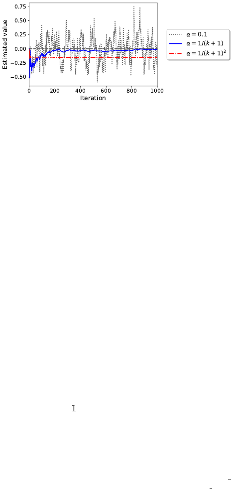
To illustrate what “suitable choice” might mean in practice, let us distill the
issue down to its essence and consider the process that estimates the mean of a
distribution ν ∈P
1
(R) according to the incremental update
V
k+1
= (1 −α
k
)V
k
+ α
k
R
k
, (6.20)
where (
R
k
)
k≥0
are i.i.d. random variables distributed according to
ν
. For concrete-
ness, let us assume that
ν
=
N
(0
,
1), so that we would like (
V
k
)
k≥0
to converge
to 0.
Suppose that the initial estimate is
V
0
= 0 (the desired solution) and consider
three step size schedules:
α
k
= 0
.
1,
α
k
=
1
/k+1
, and
α
k
=
1
/(k+1)
2
. Figure 6.1 illus-
trates the sequences of estimates obtained by applying the incremental update
with each of these schedules and a single, shared sequence of realizations of the
random variables (R
k
)
k≥0
.
The
1
/k+1
schedule corresponds to the right step size schedule for the incre-
mental Monte Carlo algorithm (Section 3.2), and accordingly, we observe that it
Draft version.
Incremental Algorithms 175
Figure 6.1
The behavior of a simple incremental update rule 6.20 for estimating the expected value
of a normal distribution. Different curves represent the sequence of estimates obtained
from different step size schedules. The ground truth (
V
= 0) is indicated by the dashed
line.
is converging to the correct expected value.
51
By contrast, the constant schedule
continues to exhibit variations over time, as the noise is not sufficiently averaged
out. The quadratic schedule (
1
/(k+1)
2
) decreases too quickly and the algorithm
settles on an incorrect prediction.
To prove the convergence of algorithms that fit the template described in
Section 6.5, we will require that the sequence of step sizes satisfies the Robbins–
Monro conditions (Robbins and Monro 1951). These conditions formalize the
range of step sizes that are neither too small nor too large and hence guarantee
that the algorithm must eventually find the solution
U
∗
. As with the source state
X
k
, the step size
α
k
at a given time
k
may be random, and its distribution may
depend on
X
k
,
X
0:k−1
, α
0:k−1
,
and
Y
0:k−1
but not the sample experience
Y
k
. As in
the previous section, these conditions should hold with probability 1.
Condition 1: not too small.
In the example above, taking
α
k
=
1
/(k+1)
2
results
in premature convergence of the estimate (to the wrong solution). This is because
when the step sizes decay too quickly, the updates made by the algorithm may
not be of large enough magnitude to reach the fixed point of interest. To avoid
this situation, we require that (α
k
)
k≥0
satisfy
X
k≥0
α
k {X
k
= x}
= ∞, for all x ∈X.
Implicit in this assumption is also the idea that every state should be updated
infinitely often. This assumption is violated, for example, if there is a state
x
51.
In our example,
V
k
is the average of
k
i.i.d. normal random variables and is itself normally
distributed. Its standard deviation can be computed analytically and is equal to
1
/
√
k
(
k ≥
1). This
implies that after
k
= 1000 iterations, we expect
V
k
to be in the range
±
3
×
1
/
√
k
=
±
0
.
111, because
99.7 percent of a normal random variable’s probability is within three standard deviations of its
mean. Compare with Figure 6.1.
Draft version.

176 Chapter 6
and time
K
after which
X
k
, x
, for all
k ≥K
. For a reasonably well-behaved
distribution of source states, this condition is satisfied for constant step sizes,
including
α
k
= 1: in the absence of noise, it is possible to make rapid progress
toward the fixed point. On the other hand, it disallows α
k
=
1
/(k+1)
2
, since
∞
X
k=0
1
(k + 1)
2
=
π
2
6
< ∞.
Condition 2: not too large.
Figure 6.1 illustrates how, with a constant step
size and in the presence of noise, the estimate
U
k
(
x
) continues to vary substan-
tially over time. To avoid this issue, the step size should be decreased so that
individual updates result in progressively smaller changes in the estimate. To
achieve this, the second requirement on the step size sequence (α
k
)
k≥0
is
X
k≥0
α
2
k
{X
k
= x}
< ∞, for all x ∈X.
In reinforcement learning, a simple step size schedule that satisfies both of
these conditions is
α
k
=
1
N
k
(X
k
) + 1
, (6.21)
where
N
k
(
x
) is the number of updates to a state
x
up to but not including
algorithm time
k
. We encountered this schedule in Section 3.2 when deriving
the incremental Monte Carlo algorithm. As will be shown in the following
sections, this schedule is also sufficient for the convergence of TD and CTD
algorithms.
52
Exercise 6.7 asks you to verify that Equation 6.21 satisfies the
Robbins–Monro conditions and investigates other step size sequences that also
satisfy these conditions.
6.7 Overview of Convergence Analysis
Provided that an incremental algorithm satisfies the template laid out in Section
6.5, with a step size schedule that satisfies the Robbins–Monro conditions,
we can prove that the sequence of estimates produced by this algorithm must
converge to the fixed point
U
∗
of the implied operator
O
. Before presenting the
proof in detail, we illustrate the main bounding-box argument underlying the
proof.
Let us consider a two-dimensional state space
X
=
{x
1
, x
2
}
and an incre-
mental algorithm for estimating a 1-dimensional quantity (
m
= 1). As per the
template, we consider a contractive operator
O
:
R
X
→R
X
given by
OU
=
52.
Because the process of bootstrapping constructs sample targets that are not in general unbiased
with regards to the value function
V
π
, the optimal step size schedule for TD learning decreases at a
rate that is slower than
1
/k. See bibliographical remarks.
Draft version.
Incremental Algorithms 177
0
.
8
U
(
x
2
)
,
0
.
8
U
(
x
2
)
; note that the fixed point of
O
is
U
∗
= (0
,
0). At each
time step, a source state (
x
1
or
x
2
) is chosen uniformly at random and the
corresponding estimate is updated. The step sizes are
α
k
= (
k
+ 1)
−0.7
, satisfying
the Robbins–Monro conditions.
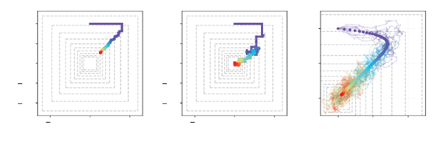
Suppose first that the sample target is noiseless. That is,
ˆ
O(U
k
, X
k
, Y
k
) = 0.8U
k
(x
2
).
In this case, each iteration of the algorithm contracts along a particular
coordinate. Figure 6.2a illustrates a sequence (
U
k
)
k≥0
defined by the update
equations
U
k+1
(X
k
) = (1 −α
k
)U
k
(X
k
) + α
k
ˆ
O(X
k
, U
k
, Y
k
)
U
k+1
(x) = U
k
(x), x , X
k
.
As shown in the figure, the algorithm makes steady (if not direct) progress
toward the fixed point with each update. To prove that (
U
k
)
k≥0
converges to
U
∗
, we first show that the error
kU
k
−U
∗
k
∞
is bounded by a fixed quantity
for all
k ≥
0 (indicated by the outermost dashed-line square around the fixed
point
U
∗
= 0 in Figure 6.2a). The argument then proceeds inductively: if
U
k
lies
within a given radius of the fixed point for all
k
greater than some
K
, then there
is some
K
0
≥K
for which, for all
k ≥K
0
, it must lie within the next smallest
dashed-line square. We will see that this follows by contractivity of
O
and the
first Robbins–Monro condition. Provided that the diameter of these squares
shrinks to zero, then this establishes convergence of U
k
to U
∗
.
Now consider adding noise to the sample target, such that
ˆ
O(U
k
, X
k
, Y
k
) = 0.8U
k
(y) + w
k
.
For concreteness, let us take
w
k
to be an independent random variable with dis-
tribution
U
([
−
1
,
1]). In this case, the behavior of the sequence (
U
k
)
k≥0
is more
complicated (Figure 6.2b). The sequence (
U
k
)
k≥0
no longer follows a neat path
to the fixed point but can behave somewhat more erratically. Nevertheless, the
long-term behavior exhibited by the algorithm bears similarity to the noiseless
case: overall, progress is made toward the fixed point U
∗
.
The proof of convergence follows the same pattern as for the noiseless case:
prove inductively that if
kU
k
−U
∗
k
∞
is eventually bounded by some fixed
quantity
B
l
∈R
, then
kU
k
−U
∗
k
∞
is eventually bounded by a smaller quantity
B
l+1
. As in the noiseless case, this argument is depicted by the concentric squares
in Figure 6.2c. Again, if these diameters shrink to zero, this also establishes
convergence of U
k
to U
∗
.
Draft version.

178 Chapter 6
Because noise can increase the error between the estimate
U
k
and the fixed
point
U
∗
at any given time step, to guarantee convergence we need to pro-
gressively decrease the step size
α
k
. The second Robbins–Monro condition is
sufficient for this purpose, and with it the inductive step can be proven with a
more delicate argument. One additional challenge is that the base case (that
sup
k≥0
kU
k
−U
∗
k
∞
< ∞
) is no longer immediate; a separate argument is required
to establish this fact. This property is called the stability of the sequence (
U
k
)
k≥0
and is often one of the harder aspects of the proof of convergence of incremental
algorithms.
We conclude this section with a result that is crucial in understanding the
influence of noise in the algorithm. In the analysis carried out in this chapter, it
is the only result whose proof requires tools from advanced probability theory.
53
Proposition 6.4.
Let (
Z
k
)
k≥0
be a sequence of random variables taking
values in
R
m
and (
α
k
)
k≥0
be a collection of step sizes. Given
¯
Z
0
= 0, consider
the sequence defined by
¯
Z
k+1
= (1 −α
k
)
¯
Z
k
+ α
k
Z
k
.
Suppose that the following conditions hold with probability 1:
E[Z
k
| Z
0:k−1
, α
0:k
] = 0 , sup
k≥0
E[kZ
k
k
2
| Z
0:k−1
, α
0:k
] < ∞,
∞
X
k=0
α
k
= ∞,
∞
X
k=0
α
2
k
< ∞.
Then
¯
Z
k
→0 with probability 1. 4
The proof is given in Remark 6.2; here, we provide some intuition that can
be gleaned without consulting the proof.
First, parallels can be drawn with the strong law of large numbers. Expanding
the definition of
¯
Z
k
yields
¯
Z
k
= (1 −α
k
) ···(1 −α
1
)α
0
Z
0
+ (1 −α
k
) ···(1 −α
2
)α
1
Z
1
+ ···+ α
k
Z
k
.
Thus,
¯
Z
k
is a weighted average of the mean-zero terms (
Z
l
)
k
l=0
. If
α
k
=
1
/k+1
, then
we obtain the usual uniformly weighted average that appears in the strong law of
large numbers. We also note that unlike the standard strong law of large numbers,
the noise terms (
Z
l
)
k
l=0
are not necessarily independent. Nevertheless, it seems
reasonable that this sequence should exhibit similar behavior to the averages that
appear in the strong law of large numbers. This also provides further intuition
53.
Specifically, the supermartingale convergence theorem; the result is a special case of the
Robbins–Siegmund theorem (Robbins and Siegmund 1971).
Draft version.
Incremental Algorithms 179
(a) (b) (c)
1 0 1
U(x
1
)
1.0
0.5
0.0
0.5
1.0
U(x
2
)
1 0 1
U(x
1
)
1.0
0.5
0.0
0.5
1.0
U(x
2
)
0.0 0.5 1.0
U(x
1
)
0.0
0.5
1.0
U(x
2
)
Figure 6.2
(a)
Example behavior of the iterates (
U
k
)
k≥0
in the noiseless case. The color scheme
indicates the iteration number from purple (
k
= 0) through to red (
k
= 1000).
(b)
Example
behavior of the iterates (
U
k
)
k≥0
in the general case.
(c)
Behavior of iterates for ten random
seeds, with the noiseless (expected) behavior overlaid.
for the conditions of Proposition 6.4. If the variance of individual noise terms
α
k
Z
k
is too great, the weighted average may not “settle down” as the number of
terms increases. Similarly, if
P
∞
k=0
α
k
is too small, the initial noise term
Z
0
will
have too large an influence over the weighted average, even as k →∞.
Second, for readers familiar with stochastic gradient descent, we can rewrite
the update scheme as
¯
Z
k+1
=
¯
Z
k
+ α
k
(−
¯
Z
k
+ Z
k
) .
This is a stochastic gradient update for the loss function
L
(
¯
Z
k
) =
1
/2k
¯
Z
k
k
2
(the
minimizer of which is the origin). The negative gradient of this loss is
−
¯
Z
k
,
Z
k
is a mean-zero perturbation of this gradient, and
α
k
is the step size used in the
update. Proposition 6.4 can therefore be interpreted as stating that stochastic
gradient descent on this specific loss function converges to the origin, under
the required conditions on the step sizes and noise. It is perhaps surprising
that understanding the behavior of stochastic gradient descent in this specific
setting is enough to understand the general class of algorithms expressed by
Equation 6.18.
6.8 Convergence of Incremental Algorithms*
We now provide a formal run-through of the arguments of the previous section
and explain how they apply to temporal-difference learning algorithms. We
begin by introducing some notation to simplify the argument. We first define a
Draft version.
180 Chapter 6
per-state step size that incorporates the choice of source state X
k
:
α
k
(x) =
α
k
if x = X
k
0 otherwise,
w
k
(x) =
ˆ
O(U
k
, X
k
, Y
k
) −(OU
k
)(X
k
) if x = X
k
0 otherwise.
This allows us to recursively define (U
k
)
k≥0
in a single equation:
U
k+1
(x) = (1 −α
k
(x))U
k
(x) + α
k
(x)
(OU
k
)(x) + w
k
(x)
. (6.22)
Equation 6.22 encapsulates all of the random variables – (
X
k
)
k≥0
, (
Y
k
)
k≥0
, (
α
k
)
k≥0
– which together determine the sequence of estimates (U
k
)
k≥0
.
It is useful to separate the effects of the noise into two separate cases: one
in which the noise has been “processed” by an application of the contractive
mapping
O
and one in which the noise has not been passed through this mapping.
To this end, we introduce the cumulative external noise vectors (
W
k
(
x
) :
k ≥
0
, x ∈X
). These are random vectors, with each
W
k
(
x
) taking values in
R
m
,
defined by
W
0
(x) = 0 , W
k+1
(x) = (1 −α
k
(x))W
k
(x) + α
k
(x)w
k
(x) .
We also introduce the sigma-algebras
F
k
=
σ
(
X
0:k
, α
0:k
, Y
0:k−1
); these encode
the information available to the learning agent just prior to sampling
Y
k
and
applying the update rule to produce U
k+1
.
We now list several assumptions we will require of the algorithm to establish
the convergence result. Recall that
k·k
is the base norm identified in Section
6.5, which gives rise to the supremum extension
k·k
∞
. In particular, we assume
that O is a β-contraction mapping in the metric induced by k·k
∞
.
Assumption 6.5
(Robbins–Monro conditions)
.
For each
x ∈X
, the step sizes
(α
k
(x))
k≥0
satisfy
P
k≥0
α
k
(x) = ∞ and
P
k≥0
α
k
(x)
2
< ∞ with probability 1. 4
The second assumption encompasses the mean-zero condition described in
Section 6.5 and introduces an additional condition that the variance of this noise,
conditional on the state of the algorithm, does not grow too quickly.
Assumption 6.6.
The noise terms (
w
k
(
x
) :
k ≥
0
, x ∈X
) satisfy
E
[
w
k
(
x
)
|F
k
] =
0 with probability 1, and
E
[
kw
k
(
x
)
k
2
|F
k
]
≤C
1
+
C
2
kU
k
k
2
∞
w.p. 1, for some
constants C
1
, C
2
≥0, for all x ∈X and k ≥0. 4
We would like to use Proposition 6.4 to show that the cumulative external
noise (
W
k
(
x
))
k≥0
is well behaved, and then use this intermediate result to estab-
lish the convergence of the sequence (
U
k
)
k≥0
itself. The proposition is almost
applicable to the sequence (
W
k
(
x
))
k≥0
. The difficulty is that the proposition
stipulates that the individual noise terms
Z
k
have bounded variance, whereas
Assumption 6.6 only bounds the conditional expectation of
kw
k
(
x
)
k
2
in terms of
kU
k
k
2
∞
, which a priori may be unbounded. Unfortunately, in temporal-difference
Draft version.

Incremental Algorithms 181
learning algorithms, the update variance typically does scale with the magnitude
of current estimates, so this is not an assumption that we can weaken. To get
around this difficulty, we first establish the boundedness of the sequence (
U
k
)
k≥0
,
as described informally in the previous section, often referred to as stability in
the stochastic approximation literature.
Proposition 6.7.
Suppose Assumptions 6.5 and 6.6 hold. Then there is a
finite random variable
B
such that
sup
k≥0
kU
k
k
∞
< B
with probability 1.
4
Proof.
The idea of the proof is to work with a “renormalized” version of the
noises (
w
k
(
x
))
k≥0
to which Proposition 6.4 can be applied. First, we show that
the contractivity of
O
means that when
U
is sufficiently far from 0,
O
contracts
the iterate back toward 0. To make this precise, we first observe that
kOUk
∞
≤kOU −U
∗
k
∞
+ kU
∗
k
∞
≤βkU −U
∗
k
∞
+ kU
∗
k
∞
≤βkUk
∞
+ D ,
where
D
= (1 +
β
)
kU
∗
k
∞
. Let
¯
B >
D
/1−β
so that
¯
B > β
¯
B
+
D
, and define
ψ ∈
(
β,
1)
by β
¯
B + D = ψ
¯
B. Now that that for any U with kUk
∞
≥
¯
B, we have
kOUk
∞
≤βkUk
∞
+ D = βkUk
∞
+ (ψ −β)
¯
B ≤βkUk
∞
+ (ψ −β)kUk
∞
= ψkUk
∞
.
Second, we construct a sequence of bounds (
¯
B
k
)
k≥0
related to the iterates (
U
k
)
k≥0
as follows. It will be convenient to introduce 1 +
ε
=
ψ
−1
, the inverse of the
contraction factor ψ above. Take
¯
B
0
= max(
¯
B, kU
0
k
∞
), and iteratively define
¯
B
k+1
=
¯
B
k
if kU
k+1
k
∞
≤(1 + ε)
¯
B
k
min{(1 + ε)
l
¯
B
0
: l ∈N
+
, kU
k+1
k
∞
≤(1 + ε)
l
¯
B
0
} otherwise .
Thus, the (
¯
B
k
)
k≥0
define a kind of soft “upper envelope” on (
kU
k
k
∞
)
k≥0
, which
are only updated when a norm exceeds the previous bound
¯
B
k
by a factor at
least (1 + ε). Note that (kU
k
k
∞
)
k≥0
is unbounded if and only if
¯
B
k
→∞.
We now use the (
¯
B
k
)
k≥0
to define a “renormalized” noise sequence (
˜w
k
)
k≥0
to which Proposition 6.4 can be applied. We set
˜w
k
=
w
k
/
¯
B
k
, and define
˜
W
k
iteratively by
˜
W
0
= w
0
, and
˜
W
k+1
(x) = (1 −α
k
(x))
˜
W
k
(x) + α
k
(x) ˜w
k
(x) .
By Assumption 6.6, we still have
E
[
˜w
k
| F
k
] = 0 and obtain that
E
[
k˜w
k
k
2
∞
| F
k
]
is uniformly bounded. Using Assumption 6.5, Proposition 6.4 now applies, and
we deduce that
˜
W
k
→0 with probability 1.
In particular, there is a (random) time
K
such that
k
˜
W
k
(
x
)
k< ε
for all
k ≥K
and
x ∈X
. Now supposing
¯
B
k
→∞
, we may also take
K
so that
kU
K
k
∞
≤
¯
B
K
.
We will now prove by induction that for all
k ≥K
, we have both
kU
k
k
∞
≤
(1 +
ε
)
¯
B
K
and
kU
k
−W
k
k
∞
<
¯
B
K
; the base case is clear from the above. For the
Draft version.

182 Chapter 6
inductive step, suppose for some
k ≥K
, we have both
kU
k
k
∞
≤
(1 +
ε
)
¯
B
K
and
kU
k
−W
k
k
∞
<
¯
B
K
. Now observe that
kU
k+1
(x) −W
k+1
(x)k
=k(1 −α
k
(x))U
k
(x) + α
k
(x)(OU
k
)(x) + α
k
(x)w
k
(x) −W
k+1
(x)k
≤(1 −α
k
(x))kU
k
(x) −W
k
(x)k+ α
k
(x)k(OU
k
)(x)k
≤(1 −α
k
(x))
¯
B
K
+ α
k
(x)(βkU
k
k
∞
+ D)
≤(1 −α
k
(x))
¯
B
K
+ α
k
(x)ψ(1 + ε)
¯
B
K
≤
¯
B
K
.
And additionally,
kU
k+1
k
∞
≤kU
k+1
−W
k+1
k
∞
+ kW
k+1
k
∞
≤
¯
B
K
+ ε
¯
B
K
= (1 + ε)
¯
B
K
as required.
We can now establish the convergence of the cumulative external noise.
Proposition 6.8.
Suppose Assumptions 6.5 and 6.6 hold. Then the external
noise W
k
(x) converges to 0 with probability 1, for each x ∈X. 4
Proof.
By Proposition 6.7, there exists a finite random variable
B
such that
kU
k
k
∞
≤B
for all
k ≥
0. We therefore have
E
[
kw
k
(
x
)
k
2
|F
k
]
≤C
1
+
C
2
B
2
=
:
B
0
w.p. 1 for all
x ∈X
and
k ≥
0, by Assumption 6.6. Proposition 6.4 therefore
applies to give the conclusion.
With this result in hand, we now prove the central result of this section,
using the stability result as the base case for the inductive argument intuitively
explained above.
Theorem 6.9.
Suppose Assumptions 6.5 and 6.6 hold. Then
U
k
→U
∗
with
probability 1. 4
Proof.
By Proposition 6.7, there is a finite random variable
B
0
such that
kU
k
−
U
∗
k
∞
< B
0
for all
k ≥
0 w.p. 1. Let
ε >
0 such that
β
+ 2
ε <
1; we will show by
induction that if
B
l
= (
β
+ 2
ε
)
B
l−1
for all
l ≥
1, then for each
l ≥
0, there is a
(possibly random) finite time
K
l
such that
kU
k
−U
∗
k
∞
< B
l
for all
k ≥K
l
, which
proves the theorem.
To prove this claim by induction, let
l ≥
0 and suppose there is a random
finite time
K
l
such that
kU
k
−U
∗
k
∞
< B
l
for all
k ≥K
l
w.p. 1. Now let
x ∈X
, and
Draft version.

Incremental Algorithms 183
k ≥K
l
. We have
U
k+1
(x) −U
∗
(x) −W
k+1
(x)
= (1 −α
k
(x))U
k
(x) + α
k
(x)((OU
k
)(x) + w
k
(x))
−U
∗
(x) −(1 −α
k
(x))W
k
(x) −α
k
(x)w
k
(x)
= (1 −α
k
(x))(U
k
(x) −U
∗
(x) −W
k
(x)) + α
k
(x)((OU
k
)(x) −U
∗
(x)) .
Since
O
is a contraction mapping under
k·k
∞
with fixed point
U
∗
and con-
traction modulus
β
, we have
k
(
OU
k
)(
x
)
−U
∗
(
x
)
k≤βkU
k
−U
∗
k
∞
< βB
l
, and
so
kU
k+1
(x) −U
∗
(x) −W
k+1
(x)k≤(1 −α
k
(x))kU
k
(x) −U
∗
(x) −W
k
(x)k+α
k
(x)βB
l
.
Letting ∆
k
(x) = kU
k
(x) −U
∗
(x) −W
k
(x)k, we then have
∆
k+1
(x) ≤(1 −α
k
(x))∆
k
(x) + α
k
(x)βB
l
=⇒ ∆
k+1
(x) −βB
l
≤(1 −α
k
(x))(∆
k
(x) −βB
l
) .
Telescoping this inequality from K
l
to k yields
∆
k+1
(x) −βB
l
≤
k
Y
s=K
l
(1 −α
s
(x))
(∆
K
l
(x) −βB
l
) .
If ∆
K
l
(
x
)
−βB
l
≤
0, then ∆
k
(
x
)
≤βB
l
for all
k ≥K
l
. If not, then we can use the
inequality 1 −x ≤e
−x
(applied to x = α
k
≥0) to deduce
∆
k+1
(x) −βB
l
≤exp
−
k
X
s=K
l
α
k
(x)
(∆
K
l
(x) −βB
l
) ,
and since
P
s≥0
α
s
(
x
) =
∞
by assumption, the right-hand side tends to 0. There-
fore, there exists a random finite time after which ∆
k
(
x
)
≤
(
β
+
ε
)
B
l
. Since
X
is
finite, there is a random finite time after which this holds for all
x ∈X
. Finally,
since
W
k
(
x
)
→
0 under
k·k
for all
x ∈X
w.p. 1 by Proposition 6.8, there is a
random finite time after which
kW
k
(
x
)
k≤εB
l
for all
x ∈X
. Letting
K
l+1
≥K
l
be
the maximum of all these random times, we therefore have that for
k ≥K
l+1
, for
all x ∈X,
kU
k
(x) −U
∗
(x)k≤kU
k
(x) −U
∗
(x) −W
k
(x)k+ kW
k
(x)k≤(β + ε)B
l
+ εB
l
= B
l+1
,
as required.
6.9 Convergence of Temporal-Difference Learning*
We can now apply Theorem 6.9 to demonstrate the convergence of the sequence
of value function estimates produced by TD learning. Formally, we consider a
stream of sample transitions (
X
k
, A
k
, R
k
, X
0
k
)
k≥0
, along with associated step sizes
Draft version.
184 Chapter 6
(α
k
)
k≥0
, that satisfy the Robbins–Monro conditions (Assumption 6.5) and give
rise to zero-mean noise terms (Assumption 6.6). More precisely, we assume
there are sequences of functions (
ξ
k
)
k≥0
and (
ν
k
)
k≥0
such that our sample model
takes the following form (for k ≥0):
X
k
|(X
0:k−1
, A
0:k−1
, R
0:k−1
, X
0
0:k−1
, α
0:k−1
)∼ξ
k
X
0:k−1
, A
0:k−1
, R
0:k−1
, X
0
0:k−1
, α
0:k−1
;
α
k
|(X
0:k
, A
0:k−1
, R
0:k−1
, X
0
0:k−1
, α
0:k−1
)∼ν
k
X
0:k
, A
0:k−1
, R
0:k−1
, X
0
0:k−1
, α
0:k−1
;
A
k
|
X
0:k
, A
0:k−1
, R
0:k−1
, X
0
0:k−1
, α
0:k
∼π( · | X
k
);
R
k
|
X
0:k
, A
0:k
, R
0:k−1
, X
0
0:k−1
, α
0:k
∼P
R
( · | X
k
, A
k
);
X
0
k
|
X
0:k
, A
0:k
, R
0:k
, X
0
0:k−1
, α
0:k
∼P
X
( · | X
k
, A
k
) . (6.23)
A generative, or algorithmic, perspective on this model is that at each update step
k
, a source state
X
k
and step size
α
k
are selected on the basis of all previously
observed random variables (possibly using an additional source of randomness
to make this selection), and the variables (
A
k
, R
k
, X
0
k
) are sampled according
to
π
and the environment dynamics, conditionally independent of all random
variables already observed given
X
k
. Readers may compare this with the model
equations in Section 2.3 describing the joint distribution of a trajectory generated
by following the policy
π
. As discussed in Sections 6.5 and 6.6, this is fairly
flexible model that allows us to analyze a variety of learning schemes.
Theorem 6.10.
Consider the value function iterates (
V
k
)
k≥0
defined by
some initial estimate V
0
and satisfying
V
k+1
(X
k
) = (1 −α
k
)V
k
(X
k
) + α
k
R
k
+ V
k
(X
0
k
)
V
k+1
(x) = V
k
(x) if x , X
k
,
where (X
k
, A
k
, R
k
, X
0
k
)
k≥0
is a sequence of transitions. Suppose that:
(a)
The source states (
X
k
)
k≥0
and step sizes (
α
k
)
k≥0
satisfy the Robbins–
Monro conditions: w.p. 1, for all x ∈X,
∞
X
k=0
α
k {X
k
= x}
= ∞,
∞
X
k=0
α
2
k
{X
k
= x}
< ∞.
(b)
The joint distribution of (
X
k
, A
k
, R
k
, X
0
k
)
k≥0
is an instance of the
sampling model expressed in Equation 6.23.
(c)
The reward distributions for all state-action pairs have finite variance.
Then V
k
→V
π
with probability 1. 4
Theorem 6.10 gives formal meaning to our earlier assertion that the conver-
gence of incremental reinforcement learning algorithms can be guaranteed for a
Draft version.

Incremental Algorithms 185
variety of source state distributions. Interestingly enough, the condition on the
source state distribution appears only implicitly, through the Robbins–Monro
conditions: effectively, what matters is not so much when the states are updated
but rather the “total amount of step size” by which the estimate may be moved.
Proof.
We first observe that the temporal-difference algorithm described in
the statement is an instance of the abstract algorithm described in Section 6.5,
by taking
U
k
=
V
k
,
m
= 1,
O
=
T
π
,
Y
k
= (
A
k
, R
k
, X
0
k
), and
ˆ
O
(
U
k
, X
k
, Y
k
) =
R
k
+
γV
k
(
X
0
k
). The base norm
k·k
is simply the absolute value on
R
. In this case,
O
is
a
γ
-contraction on
R
X
by Proposition 4.4, with fixed point
V
π
, and the noise
w
k
is equal to
R
k
+
γV
k
(
X
0
k
)
−
(
T
π
U
k
)(
X
k
), by the decomposition in Equation 6.5.
It therefore remains to check that Assumptions 6.5 and 6.6 hold; Theorem 6.9
then applies to give the result. Assumption 6.5 is immediate from the conditions
of the theorem. To see that Assumption 6.6 holds, first note that
E[w
k
|F
k
] = E
π
[R
k
+ γV
k
(X
0
k
) −(T
π
V
k
)(X
k
) |F
k
]
= E
π
[R
k
+ γV
k
(X
0
k
) −(T
π
V
k
)(X
k
) |X
k
, V
k
]
= 0 ,
since conditional on (
X
k
, V
k
), the expectation of
R
+
γV
k
(
X
0
k
) is (
T
π
V
k
)(
X
k
).
Additionally, we note that
E
|w
k
|
2
|F
k
= E
|w
k
|
2
|X
k
, V
k
= E
|R + γV
k
(X
0
k
) −(T
π
V
k
)(X
k
)|
2
|X
k
, V
k
≤2
E
|R + γV
k
(X
0
k
)|
2
|X
k
, V
k
+ (T
π
V
k
)(X
k
)
2
≤C
1
+ C
2
kV
k
k
2
∞
,
for some C
1
, C
2
> 0.
6.10 Convergence of Categorical Temporal-Difference Learning*
Let us now consider proving the convergence of categorical TD learning
by means of Theorem 6.9. Writing CTD in terms of a sequence of return
distribution estimates, we have
η
k+1
(X
k
) = (1 −α
k
)η
k
(X
k
) + α
k
Π
c
(b
R
k
,γ
)
#
η(X
0
k
)
η
k+1
(x) = η
k
(x) if x , X
k
. (6.24)
Following the principles of the previous section, we may decompose the update
at X
k
into an operator term and a noise term:
η
k+1
(X
k
) = (1 −α
k
)η
k
(X
k
) (6.25)
+ α
k
(Π
c
T
π
η)(X
k
)
| {z }
(OU)(X
k
)
+ Π
c
(b
R
k
,γ
)
#
η(X
0
k
) −(Π
c
T
π
η)(X
k
)
| {z }
w
k
.
Draft version.
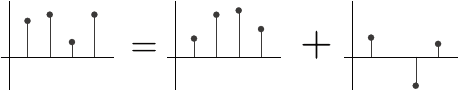
186 Chapter 6
Assuming that
R
k
and
X
0
k
are drawn appropriately, this decomposition is sensible
by virtue of Proposition 6.2, in the sense that the expectation of the sample
target is the projected distributional Bellman operator:
E
π
Π
c
(b
R
k
,γ
)
#
η(X
0
k
)
| X
k
= x
= (Π
c
T
π
η
(x) for all x . (6.26)
With this decomposition, the noise term is not a probability distribution but
rather a signed distribution; this is illustrated in Figure 6.3. Informally speaking,
a signed distribution may assign negative “probabilities” and may not integrate
to one (we will revisit signed distributions in Chapter 9). Based on Proposition
6.2, we may intuit that
w
k
is mean-zero noise, where “zero” here is to be
understood as a special signed distribution.
(a) Categorical TD target (b) Expected update (c) Mean-zero noise
Figure 6.3
The sample target in a categorical TD update
(a)
can be decomposed into an expected
update specified by the operator Π
c
T
π
(b) and a mean-zero signed distribution (c).
However, expressing the CTD update rule in terms of signed distributions
is not sufficient to apply Theorem 6.9. This is because the theorem requires
that the iterates
U
k
(
x
)
k≥0
be elements of
R
m
, whereas (
η
k
(
x
))
k≥0
are proba-
bility distributions. To address this issue, we leverage the fact that categorical
distributions are represented by a finite number of parameters and view their
cumulative distribution functions as in vectors in R
m
.
Recall that
F
X
C,m
is the space of
m
-categorical return distribution functions.
To invoke Theorem 6.9, we construct an isometry
I
between
F
X
C,m
and a certain
subset of R
X×m
. For a categorical return function η ∈F
X
C,m
, write
I(η) =
F
η(x)
(θ
i
) : x ∈X, i ∈{1, . . . , m}
∈R
X×m
,
where as before
θ
1
, . . . , θ
m
denotes the locations of the
m
particles whose prob-
abilities are parameterized in
F
C,m
. The isometry
I
maps return functions
to elements of
R
X×m
describing the corresponding cumulative distribution
functions (CDFs), evaluated at these particles. The image of F
X
C,m
under I is
R
X
I
= {z ∈R
m
: 0 ≤z
1
≤···≤z
m
= 1}
X
.
Draft version.

Incremental Algorithms 187
The inverse map
I
−1
: R
X
I
→F
X
C,m
maps vectors describing the cumulative distribution functions of categorical
return functions back to their distributions.
With this construction, the metric induced by the
L
2
norm
k·k
2
over
R
m
is
proportional to the Cramér distance between probability distributions and is
readily extended to R
X×m
. That is, for η, η
0
∈F
X
C,m
, we have
I(η) −I(η
0
)
2,∞
= sup
x∈X
(I(η))(x) −(I(η
0
))(x)
2
=
1
ς
m
2
(η, η
0
).
We will prove the convergence of the sequence (
η
k
)
k≥0
defined by Equation 6.24
to the fixed point of the projected operator Π
c
T
π
by applying Theorem 6.9 to
the sequence (
I
(
η
k
))
k≥0
and the
L
2
metric and arguing (by isometry) that the
original sequence must also converge. An important additional property of
I
is
that it commutes with expectations, in the following sense.
Lemma 6.11.
The isometry
I
:
F
X
C,m
→R
X
I
is an affine map. That is, for any
η, η
0
∈F
X
C,m
and α ∈[0, 1],
I(αη + (1 −α)η
0
) = αI(η) + (1 −α)I(η
0
) .
As a result, if η is a random return-distribution function, then we have
E[I(η)] = I(E[η]) . 4
Theorem 6.12.
Let
m ≥
2 and consider the return function iterates (
η
k
)
k≥0
generated by Equation 6.24 from some possibly random
η
0
. Suppose that:
(a)
The source states (
X
k
)
k≥0
and step sizes (
α
k
)
k≥0
satisfy the Robbins–
Monro conditions: w.p. 1, for all x ∈X,
∞
X
k=0
α
k {X
k
= x}
= ∞,
∞
X
k=0
α
2
k
{X
k
= x}
< ∞.
(b)
The joint distribution of (
X
k
, A
k
, R
k
, X
0
k
)
k≥0
is an instance of the
sampling model expressed in Equation 6.23.
Then, with probability 1,
η
k
→ ˆη
π
c
with respect to the supremum Cramér
distance
2
, where
ˆη
π
c
is the unique fixed point of the projected operator
Π
c
T
π
:
ˆη
π
c
= Π
c
T
π
ˆη
π
c
. 4
Draft version.

188 Chapter 6
Proof.
We begin by constructing a sequence (
U
k
)
k≥0
,
U
k
∈R
X
I
that parallels the
sequence of return functions (η
k
)
k≥0
. Write
O= I◦Π
c
T
π
◦I
−1
and define, for each
k ∈N
,
U
k
=
I
(
η
k
). By Lemma 5.24,
O
is a contraction with
modulus γ
1
/2
in k·k
2,∞
and we have
U
k+1
(X
k
)
= (1 −α
k
)U
k
(X
k
) + α
k
I
Π
c
(b
R
k
,γ
)
#
η(X
0
k
)
= (1 −α
k
)U
k
(X
k
) + α
k
(OU
k
)(X
k
) + IΠ
c
(b
R
k
,γ
)
#
(I
−1
U
k
)(X
0
k
) −(OU
k
)(X
k
)
| {z }
w
k
.
To see that Assumption 6.6 (bounded, mean-zero noise) holds, first note that
by Proposition 6.2 and affineness of
I
and
I
−1
from Lemma 6.11, we have
E
[
w
k
|F
k
] = 0. Furthermore,
w
k
is a bounded random variable, because each
coordinate is a difference of two probabilities and hence in the interval [
−
1
,
1].
Hence, we have E[kw
k
k
2
|F
k
] < C for some C > 0, as required.
By Banach’s theorem, the operator
O
has a unique fixed point
U
∗
. We can
thus apply Theorem 6.9 to conclude that the sequence (
U
k
)
k≥0
converges to
U
∗
,
satisfying
U
∗
= IΠ
c
T
π
I
−1
U
∗
. (6.27)
Because
I
is an isometry, this implies that (
η
k
)
k≥0
converges to
η
∗
=
I
−1
U
∗
.
Applying I
−1
to both sides of Equation 6.27, we obtain
I
−1
U
∗
= Π
c
T
π
I
−1
U
∗
.
Since Π
c
T
π
has a unique fixed point, we conclude that η
∗
= ˆη
π
c
.
The proof of Theorem 6.12 illustrates how the parameters of categorical
distributions are by design bounded, so that stability (i.e., Proposition 6.7) is
immediate. In fact, stability is also immediate for TD learning when the reward
distributions have bounded support.
6.11 Technical Remarks
Remark 6.1.
Given a probability distribution
ν ∈P
(
R
) and a level
τ ∈
(0
,
1),
quantile regression finds a value θ
∗
∈R such that
F
ν
(θ
∗
) = τ . (6.28)
In some situations, for example when
ν
is a discrete distribution, there are
multiple values satisfying Equation 6.28. Let us write
S = {θ : F
ν
(θ) = τ}.
Draft version.

Incremental Algorithms 189
Then one can show that
S
forms an interval. We can argue that quantile regres-
sion converges to this set by noting that, for
τ ∈
(0
,
1) the expected quantile
loss
L
τ
(θ) = E
Z∼ν
|
{Z<θ}
−τ|×|Z −θ|
is convex in
θ
. In addition, for this loss, we have that for any
θ, θ
0
∈S
and
θ
00
< S
,
L
τ
(θ) = L
τ
(θ
0
) < L
τ
(θ
00
) .
Convergence follows under appropriate conditions by appealing to standard
arguments regarding the convergence of stochastic gradient descent; see, for
example, Kushner and Yin (2003). 4
Remark 6.2
(
Proof of Proposition 6.4
)
.
Our goal is to show that
k
¯
Z
k
k
2
2
behaves like a nonnegative supermartingale, from which convergence would
follow from the supermartingale convergence theorem (see, e.g., Billingsley
2012). We begin by expressing the squared Euclidean norms of the sequence
elements recursively, writing F
k
= σ(Z
0:k−1
, α
0:k
):
E[k
¯
Z
k+1
(x)k
2
2
|F
k
] = E[k(1 −α
k
)
¯
Z
k
+ α
k
Z
k
k
2
2
|F
k
]
(a)
= (1 −α
k
)
2
k
¯
Z
k
k
2
2
+ α
2
k
E[kZ
k
k
2
2
|F
k
]
(b)
≤ (1 −α
k
)
2
k
¯
Z
k
k
2
2
+ α
2
k
B
≤(1 −α
k
)k
¯
Z
k
k
2
2
+ α
2
k
B . (6.29)
Here, (a) follows by expanding the squared norm and using
E
[
Z
k
|F
k
] = 0, and
(b) follows from the boundedness of the conditional variance of the (
Z
k
)
k≥0
,
where B is a bound on such variances.
This inequality does not establish the supermartingale property, due to the
presence of the additive term
α
2
k
B
on the right-hand side. However, the ideas
behind the Robbins–Siegmund theorem (Robbins and Siegmund 1971) can be
applied to deal with this term. The argument first constructs the sequence
Λ
k
= k
¯
Z
k
k
2
2
+
k−1
X
s=0
α
k
k
¯
Z
s
k
2
2
−B
k−1
X
s=0
α
2
s
.
Inequality 6.29 above then shows that (Λ
k
)
k≥0
is a supermartingale but may
not be uniformly bounded below, meaning the supermartingale convergence
theorem still cannot be applied. Defining the stopping times
t
q
=
inf{k ≥
0 :
B
0
P
k
s=0
α
2
s
> q}
for each
q ∈N
(with the convention that
inf ∅
=
∞
), each stopped
process (Λ
k∧t
q
)
k≥0
is a supermartingale bounded below by
−q
, and hence each
such process converges w.p. 1 by the supermartingale convergence theorem.
However,
B
0
P
∞
s=0
α
2
s
< ∞
w.p. 1 by assumption, so w.p. 1
t
q
=
∞
for sufficiently
large
q
, and hence Λ
k
converges w.p. 1. Since
P
∞
k=0
α
k
=
∞
w.p. 1 by assumption,
Draft version.
190 Chapter 6
it must be the case that
k
¯
Z
k
k
2
2
→
0 as
k →
0, in order for Λ
k
to have a finite
limit, and hence we are done. Although somewhat involved, Exercise 6.13
demonstrates the necessity of this argument. 4
6.12 Bibliographical Remarks
The focus of this chapter has been in developing and analyzing single-step
temporal-difference algorithms. Further algorithmic developments include
the use of multistep returns (Sutton 1988), off-policy corrections (Precup et
al. 2000), and gradient-based algorithms (Sutton et al. 2009; Sutton et al. 2008a);
the exercises in this chapter develop a few such approaches.
6.1–6.2.
This chapter analyzes incremental algorithms through the lens of
approximating the application of dynamic programming operators. Temporal-
difference algorithms have a long history (Samuel 1959), and the idea of
incremental approximations to dynamic programming formed motivation for
several general-purpose temporal-difference learning algorithms (Sutton 1984,
1988; Watkins 1989).
Although early proofs of particular kinds of convergence for these algorithms
did not directly exploit this connection with dynamic programming (Watkins
1989; Watkins and Dayan 1992; Dayan 1992), later a strong theoretical connec-
tion was established that viewed these algorithms through the lens of stochastic
approximation theory, allowing for a unified approach to proving almost-sure
convergence (Gurvits et al. 1994; Dayan and Sejnowski 1994; Tsitsiklis 1994;
Jaakkola et al. 1994; Bertsekas and Tsitsiklis 1996; Littman and Szepesvári
1996). The unbiased estimation framework presented comes from these works,
and the second principle is based on the ideas behind two-timescale algorithms
(Borkar 1997, 2008). A broader framework based on asymptotically approxi-
mating the trajectories of differential equations is a central theme of algorithm
design and stochastic approximation theory more generally (Ljung 1977; Kusher
and Clark 1978; Borkar and Meyn 2000; Kushner and Yin 2003; Borkar 2008;
Benveniste et al. 2012; Meyn 2022).
In addition to the CTD and QTD algorithms described in this chapter, several
other approaches to incremental learning of return distributions have been
proposed. Morimura et al. (2010b) propose to update parametric density models
by taking gradients of the Kullback-Leibler divergence between the current
estimates and the result of applying the Bellman operator to these estimates.
Barth-Maron et al. (2018) also take this approach, using a representation based
on mixtures of Gaussians. Nam et al. (2021) also use mixtures of Gaussians
and minimize the Cramér distance from a multistep target, incorporating ideas
from TD(
λ
) (Sutton 1984, 1988). Gruslys et al. (2018) combine CTD with
Draft version.
Incremental Algorithms 191
Retrace(
λ
), a multistep off-policy evaluation algorithm (Munos et al. 2016).
Nguyen et al. (2021) combine the quantile representation with a loss based
on the MMD metrics described in Chapter 4. Martin et al. (2020) propose a
proximal update scheme for the quantile representation based on (regularized)
Wasserstein flows (Jordan et al. 1998; Cuturi 2013; Peyré and Cuturi 2019).
Example 6.1 is from Bellemare et al. (2016).
6.3.
The categorical temporal-difference algorithm as a mixture update was
presented by Rowland et al. (2018). This is a variant of the C51 algorithm
introduced by Bellemare et al. (2017a), which uses a projection in a mixture of
Kullback–Leibler divergence and Cramér distance. Distributional versions of
gradient temporal-difference learning (Sutton et al. 2008a; Sutton et al. 2009)
based on the categorical representation have also been explored by Qu et
al. (2019).
6.4.
The QTD algorithm was introduced by Dabney et al. (2018b). Quan-
tile regression itself is a long-established tool within statistics, introduced by
Koenker and Bassett (1978); Koenker (2005) is a classic reference on the sub-
ject. The incremental rule for estimating quantiles of a fixed distribution was in
fact proposed by Robbins and Monro (1951), in the same paper that launched
the field of stochastic approximation.
6.5.
The discussion of sequences of learning rates that result in convergence
goes back to Robbins and Monro (1951), who introduced the field of stochastic
approximation. Szepesvári (1998), for example, considers this framework in
their study of the asymptotic convergence rate of Q-learning. A fine-grained
analysis in the case of temporal-difference learning algorithms, taking finite-
time concentration into account, was undertaken by Even-Dar and Mansour
(2003); see also Azar et al. (2011).
6.6–6.10.
Our proof of Theorem 6.9 (via Propositions 6.4, 6.7, and 6.8) closely
follows the argument given by Bertsekas and Tsitsiklis (1996) and Tsitsiklis
(1994). Specifically, we adapt this argument to deal with distributional informa-
tion, rather than a single scalar value. Proposition 6.4 is a special case of the
Robbins–Siegmund theorem (Robbins and Siegmund 1971), and a particularly
clear exposition of this and related material is given by Walton (2021). We note
also that this result can also be established via earlier results in the stochastic
approximation literature (Dvoretzky 1956), as noted by Jaakkola et al. (1994).
Theorem 6.10 is classical, and results of this kind can be found in Bertsekas and
Tsitsiklis (1996). Theorem 6.12 was first proven by Rowland et al. (2018), albeit
with a monotonicity argument based on that of Tsitsiklis (1994); the argument
here is based on a contraction mapping argument to match the analysis of the
temporal-difference algorithm. For further background on signed measures, see
Doob (1994).
Draft version.
192 Chapter 6
6.13 Exercises
Exercise 6.1.
In this chapter, we argued for a correspondence between oper-
ators and incremental algorithms. This also holds true for the incremental
Monte Carlo algorithm introduced in Section 3.2. What is peculiar about the
corresponding operator? 4
Exercise 6.2.
Exercise 3.2 asked you to derive an incremental algorithm from
the n-step Bellman equation
V
π
(x) = E
π
n−1
X
t=0
γ
t
R
t
+ γ
n
V
π
(X
n
) | X
0
= x
.
Describe this process in terms of the method where we substitute random
variables with their realizations, then derive the corresponding incremental
algorithm for state-action value functions. 4
Exercise 6.3
(*)
.
The
n
-step random-variable Bellman equation for a policy
π
is given by
G
π
(x)
D
=
n−1
X
t=0
γ
t
R
t
+ γ
n
G
π
(X
n
), X
0
= x,
where the trajectory (
X
0
=
x, A
0
, R
0
, …, X
n
, A
n
, R
n
) is distributed according to
P
π
(· | X
0
= x).
(i)
Write down the distributional form of this equation and the corresponding
n-step distributional Bellman operator.
(ii)
Show that it is a contraction on a suitable subset of
P
(
R
)
X
with respect to
an appropriate metric.
(iii)
Further show that the composition of this operator with either the categori-
cal projection or the quantile projection is also a contraction mapping in the
appropriate metric.
(iv)
Using the approach described in this chapter, derive
n
-step versions of
categorical and quantile temporal-difference learning.
(v)
In the case of
n
-step CTD, describe an appropriate set of conditions that
allow for Theorem 6.9 to be used to obtain convergence to the projected
operator fixed point with probability 1. What happens to the fixed points of
the projected operators as n →∞?
4
Exercise 6.4.
Implement the quantile regression update rule (Equation 6.11).
Given an initial estimate
θ
0
= 0, visualize the sequence of estimates produced
by quantile regression for
τ ∈{
0
.
01
,
0
.
1
,
0
.
5
}
and a constant step size
α
= 0
.
01,
given samples from
Draft version.

Incremental Algorithms 193
(i) a normal distribution N(1, 2) ;
(ii) a Bernoulli distribution U({0, 1}) ;
(iii) the mixture distribution
1
3
δ
1
+
2
3
U([2, 3]) . 4
Exercise 6.5.
Let
η
0
be a
m
-quantile return-distribution function, and let
(
x, a, r, x
0
) denote a sample transition. Find a Markov decision process for
which the update rule
η(x) ←Π
q
h
(1 −α)η(x) + αη
0
(x
0
)
i
does not converge. 4
Exercise 6.6.
Implement the TD, CTD, and QTD algorithms, and use these
algorithms to approximate the value (or return) function of the quick policy on
the Cliffs domain (Example 2.9). Compare their accuracy to the ground-truth
value function and return-distribution function estimated using many Monte
Carlo rollouts, both in terms of an appropriate metric and by visually comparing
the approximations to the ground-truth functions.
Investigate how this accuracy is affected by different choices of constant step
sizes and sequences of step sizes that satisfy the requirements laid out in Section
6.6. What do you notice about the relative performance of these algorithms as
the degree of action noise p is varied?
Investigate what happens when we modify the TD algorithm by restricting
value function estimates on the interval [
−C, C
], for a suitable
C ∈R
+
. Does
this restriction affect the performance of the algorithm differently from the
restriction to [θ
1
, θ
m
] that is intrinsic to CTD? 4
Exercise 6.7.
Let (
X
k
, A
k
, R
k
, X
0
k
)
k≥0
be a random sequence of transitions such
that for each x ∈X, we have X
k
= x for infinitely many k ≥0. Show that taking
α
k
=
1
N
k
(X
k
) + 1
.
satisfies Assumption 6.5. 4
Exercise 6.8.
Theorems 6.10 and 6.12 establish convergence for state-indexed
value functions and return-distribution functions under TD and CTD learning,
respectively. Discuss how Theorem 6.9 can be used to establish convergence of
the corresponding state-action-indexed algorithms. 4
Exercise 6.9
(*)
.
Theorem 6.10 establishes that temporal-difference learning
converges for a reasonably wide parameterization of the distribution of source
states and step size schedules. Given a source state
X
k
, consider the incremental
Monte Carlo update
V
k+1
(X
k
) = (1 −α
k
)V
k
(X
k
) + α
k
G
k
Draft version.

194 Chapter 6
V
k+1
(x) = V
k
(x) if x , X
k
,
where
G
k
∼η
π
(
X
k
) is a random return. Explain how Theorem 6.10 and its proof
should be adapted to prove that the sequence (V
k
)
k≥0
converges to V
π
. 4
Exercise 6.10
(Necessity of conditions for convergence of TD learning)
.
The
purpose of this exercise is to explore the behavior of TD learning when the
assumptions of Theorem 6.10 do not hold.
(i)
Write down an MDP with a single state
x
, from which trajectories immedi-
ately terminate, and a sequence of positive step sizes (
α
k
(
x
))
k≥0
satisfying
P
k≥0
α
k
(
x
)
< ∞
, with the property that the TD update rule applied with these
step sizes produces a sequence of estimates (
V
k
)
k≥0
that does not converge
to V
π
.
(ii)
For the same MDP, write down a sequence of positive step sizes (
α
k
(
x
))
k≥0
such that
P
k≥0
α
2
k
(
x
) =
∞
, and show that the sequence of estimates (
V
k
)
k≥0
generated by TD learning with these step sizes does not converge to V
π
.
(iii)
Based on your answers to the previous two parts, for which values of
β ≥
0
do step size sequences of the form
α
k
=
1
(N
k
(X
k
) + 1)
β
lead to guaranteed TD converge, assuming all states are visited infinitely
often?
(iv)
Consider an MDP with a single state
x
, from which trajectories immedi-
ately terminate. Suppose the reward distribution at
x
is a standard Cauchy
distribution, with density
f (z) =
1
π(1 + z
2
)
.
Show that if
V
0
also has a Cauchy distribution with median 0, then for any
positive step sizes (
α
k
(
x
))
k≥0
,
V
k
has a Cauchy distribution with median
0, and hence the sequence does not converge to a constant. Hint. The
characteristic function of the Cauchy distribution is given by
s 7→exp
(
−|s|
).
(v)
(*) In the proof of Theorem 6.9, the inequality 1
−u ≤exp
(
−u
) was used
to deduce that the condition
P
k≥0
α
k
(
x
) =
∞
w.p. 1 is sufficient to guarantee
that
k
Y
l=0
(1 −α
l
(x)) →0
w.p. 1. Show that if
α
k
(
x
)
∈
[0
,
1], the condition
P
k≥0
α
k
(
x
) =
∞
w.p. 1 is
necessary as well as sufficient for the sequence
Q
k
l=0
(1
−α
l
(
x
)) to also
converge to zero w.p. 1. 4
Draft version.

Incremental Algorithms 195
Exercise 6.11.
Using the tools from this chapter, prove the convergence of
the undiscounted, finite-horizon categorical Monte Carlo algorithm (Algorithm
3.3). 4
Exercise 6.12. Recall the no-loop operator introduced in Example 4.6:
T
π
nl
V
(x) = E
π
R + γV(X
0
)
{X
0
, x}
| X = x
.
Denote its fixed point by
V
π
nl
. For a transition (
x, a, r, x
0
) and time-varying step
size α
k
∈[0, 1), consider the no-loop update rule:
V(x) ←
(1 −α
k
)V(x) + α
k
(r + γV(x
0
)) if x
0
, x,
(1 −α
k
)V(x) + α
k
r if x
0
= x
.
(i)
Demonstrate that this update rule can be derived by substitution applied to
the no-loop operator.
(ii)
In words, describe how you would modify the online, incremental first-visit
Monte Carlo algorithm (Algorithm 3.1) to learn V
π
nl
.
(iii)
(*) Provide conditions under which the no-loop update converges to
V
π
nl
,
and prove that it does converge under those conditions. 4
Exercise 6.13.
Assumption 6.5 requires that the sequence of step sizes (
α
k
(
x
) :
k ≥0, x ∈X) satisfy
∞
X
k=0
α
k
(x)
2
< ∞ (6.30)
with probability 1. For
k ≥
0, let
N
k
(
x
) be the number of times that
x
has been
updated, and let
u
k
(
x
) be the most recent time at which
x
l
=
x
,
l < k
with the
convention that u
k
(x) = 1 if N
k
(x) = 0. Consider the step size schedule
α
k+1
=
(
1
N
k
(X
k
)+1
if u
k
(X
k
) ≤
k
2
1 otherwise.
This schedule takes larger steps for states whose estimate has not been recently
updated. Suppose that
X
k
∼ξ
for some distribution
ξ
that puts positive probabil-
ity mass on all states. Show that the sequence (
α
k
)
k≥0
satisfies Equation 6.30
w.p. 1, yet there is no B ∈R for which
∞
X
k=0
α
k
(x)
2
< B
with probability 1. This illustrates the need for the care taken in the proof of
Proposition 6.4. 4
Draft version.