Distributional Dynamic Programming

Markov decision processes model the dynamics of an agent exerting control

over its environment. Once the agent’s policy is selected, a Markov decision

process gives rise to a sequential system whose behavior we would like to char-

acterize. In particular, policy evaluation describes the process of determining

the returns obtained from following a policy

. Algorithmically, this translates

into the problem of computing the value or return-distribution function given

the parameters of the Markov decision process and the agent’s policy.

Computing the return-distribution function requires being able to describe

the output of the algorithm in terms of atomic objects (depending on the pro-

gramming language, these may be bits, ﬂoating point numbers, vectors, or even

functions). This is challenging because in general, return distributions take on a

continuum of values (i.e., they are inﬁnite-dimensional objects). By contrast,

the expected return from a state

is described by a single real number. Deﬁning

an algorithm that computes return-distribution functions ﬁrst requires us to

decide how we represent probability distributions in memory, knowing that

some approximation error must be incurred if we want to keep things ﬁnite.

This chapter takes a look at diﬀerent representations of probability distribu-

tions as they relate to the problem of computing return-distribution functions.

We will see that, unlike the relatively straightforward problem of computing

value functions, there is no obviously best representation for return-distribution

functions and that diﬀerent ﬁnite-memory representations oﬀer diﬀerent advan-

tages. We will also see that making eﬀective use of diﬀerent representations

requires diﬀerent algorithms.

5.1 Computational Model

As before, we assume that the environment is described as a ﬁnite-state, ﬁnite-

action Markov decision process. We write

and

for the size of the state

and action spaces

and

. When describing algorithms in this chapter, we will

Draft version. 115

116 Chapter 5

further assume that the reward distributions

(

· | x, a

) are supported on a ﬁnite

set

of size

; we discuss a way of lifting this assumption in Remark 5.1.

Of note, having ﬁnitely many rewards guarantees the existence of an interval

[

min

, V

max

] within which the returns lie.

We measure the complexity of a

particular algorithm in terms of the number of atomic instructions or memory

words it requires, assuming that these can reasonably be implemented in a

physical computer, as described by the random-access machine (RAM) model

of computation (Cormen et al. 2001).

In classical reinforcement learning, linear algebra provides a simple algorithm

for computing the value function of a policy

. In vector notation, the Bellman

equation is

= r

+ γP

, (5.1)

where the transition function

is represented as an

-dimensional square

stochastic matrix, and

is an

-dimensional vector. With some matrix algebra,

we deduce that

= r

+ γP

⇐⇒ (I −γP

= r

⇐⇒ V

= (I −γP

)

−1

. (5.2)

The computational cost of determining

is dominated by the matrix inversion,

requiring

(

) operations. The result is exact. The matrix

and the vector

are constructed entry-wise by writing expectations as sums:

| x) =

a∈A

π(a | x)P

| x, a)

(x) =

a∈A

r∈R

π(a | x)P

(r | x, a) ×r .

When the matrix inversion is undesirable, the value function can instead be

found by dynamic programming. Dynamic programming describes a wide vari-

ety of computational methods that ﬁnd the solution to a given problem by

caching intermediate results. In reinforcement learning, the dynamic program-

ming approach for ﬁnding the value function

, also called iterative policy

evaluation, begins with an initial estimate V

∈R

and successively computes

k+1

= T

for

= 1

, . . .

, until some desired number of iterations

have been performed

or some stopping criterion is reached. This is possible because, when

X, A

, and

35.

We can always take

min

and

max

to be the smallest and largest possible rewards, respectively.

Draft version.

Distributional Dynamic Programming 117

R are all ﬁnite, the Bellman operator can be written in terms of sums:

)(x) =

a∈A

r∈R

∈X

(A = a, R = r, X

= x

| X = x)

| {z }

π(a | x)P

| x,a)P

(r | x,a)



r + γV

)



. (5.3)

A naive implementation expresses these sums as nested for loops. Since the new

value function must be computed at all states, this naive implementation requires

on the order of

operations. We can do better by implementing it

in terms of vector operations:

k+1

= r

+ γP

, (5.4)

where

is stored in memory as an

-dimensional vector. A single appli-

cation of the Bellman operator with vectors and matrices requires

(

) operations for computing

and

, and

(

) operations for the

matrix-vector multiplication. As

and

do not need to be recomputed

between iterations, the dominant cost of this process comes from the successive

matrix multiplications, requiring O(KN

) operations.

In general, the iterates (

)

k≥0

will not reach

after any ﬁnite number of

iterations. However, the contractive nature of the Bellman operator allows us to

bound the distance from any iterate to the ﬁxed point V

Proposition 5.1.

Let

∈R

be an initial value function and consider the

iterates

k+1

= T

. (5.5)

For any ε > 0, if we take

≥

log





+ log(kV

−V

∞

)

log





then for all k ≥K

, we have that

−V

∞

≤ε .

For V

= 0, the dependency on V

can be simpliﬁed by noting that

log(kV

−V

∞

) = log(kV

∞

) ≤log



max(|V

min

|, |V

max



. 4

Proof.

Since

is a contraction mapping with respect to the

∞

metric with con-

traction modulus

(Proposition 4.4), and

is its ﬁxed point (Proposition 2.12),

36.

Assuming that the number of states

is large compared to the number of actions

and

rewards

. For transition functions with special structure (sparsity, low rank, etc.), one can hope

to do even better.

Draft version.

118 Chapter 5

we have for any k ≥1

−V

∞

= kT

k−1

−T

∞

≤γkV

k−1

−V

∞

and so by induction we have

−V

∞

≤γ

−V

∞

Setting the right-hand side to be less than or equal to

and rearranging gives

the required inequality for K

From Proposition 5.1, we conclude that we can obtain an

-approximation

(

) operations, by applying the Bellman operator

times to

an initial value function

= 0. Since the iterate

can be represented as an

-dimensional vector and is the only object that the algorithm needs to store in

memory (other than the description of the MDP itself), this shows that iterative

policy evaluation can approximate V

eﬃciently.

5.2 Representing Return-Distribution Functions

Now, let us consider what happens in distributional reinforcement learning.

As with any computational problem, we ﬁrst must decide on a data structure

that our algorithms operate on. The heart of our data structure is a scheme for

representing return-distribution functions in memory. We call such a scheme a

probability distribution representation.

Deﬁnition 5.2.

A probability distribution representation

, or simply repre-

sentation, is a collection of probability distributions indexed by a parameter

from some set of allowed parameters Θ:

F =



∈P (R) : θ ∈Θ



. 4

Example 5.3.

The Bernoulli representation is the set of all Bernoulli distribu-

tions:



(1 − p)δ

+ pδ

: p ∈[0, 1]



. 4

Example 5.4.

The uniform representation is the set of all uniform distributions

on ﬁnite-length intervals:



U([a, b]) : a, b ∈R, a < b



. 4

We represent return functions using a table of probability distributions, each

associated with a given state and described in our chosen representation. For

example, a uniform return function is described in memory by a table of 2

numbers, corresponding to the upper and lower ends of the distribution at each

state. By extension, we call such a table a representation of return-distribution

Draft version.

Distributional Dynamic Programming 119

functions. Formally, for a representation

, the space of representable return

functions is F

With this data structure in mind, let us consider the procedure (introduced by

Equation 4.10) that approximates the return function

by repeatedly applying

the distributional Bellman operator:

k+1

= T

. (5.6)

Because an operator is an abstract object, Equation 5.6 describes a mathematical

procedure, rather than a computer program. To obtain the latter, we begin by

expressing the distributional Bellman operator as a sum, analogous to Equation

5.3. Recall that the distributional operator is deﬁned by an expectation over the

random variables R and X

η)(x) = E

[(b

R,γ

)

η(X

) |X = x] . (5.7)

Here, the expectation describes a mixture of pushforward distributions. By

writing this expectation in full, we ﬁnd that this mixture is given by





(x) =

a∈A

r∈R

∈X



A = a, R = r, X

= x

| X = x



r,γ

)

η(x

) . (5.8)

The pushforward operation scales and then shifts (by

and

, respectively)

the support of the probability distribution

(

), as depicted in Figure 2.5.

Implementing the distributional Bellman operator therefore requires being able

to eﬃciently perform the shift-and-scale operation and compute mixtures of

probability distributions; we caught a glimpse of what that might entail when

we derived categorical temporal-diﬀerence learning in Chapter 3.

Cumulative distribution functions allow us to rewrite Equations 5.7–5.8 in

terms of vector-like objects, providing a nice parallel with the usual vector

notation for the expected-value setting. Let us write

(

x, z

) =

η(x)

(

) to denote

the cumulative distribution function of

(

). We can equally express Equation

5.7 as

)(x, z) = E



z−R



| X = x

. (5.9)

As a weighted sum of cumulative distribution functions, Equation 5.9 is

)(x, z) =

a∈A

r∈R

∈X



A = a, R = r, X

= x

| X = x





z−r



. (5.10)

Similar to Equation 5.1, we can set

on both sides of Equation 5.10 to

obtain the linear system:

(x, z) =

a∈A

r∈R

∈X



A = a, R = r, X

= x

| X = x





z−r



37.

With Chapter 4 in mind, note that we are overloading operator notation when we apply

collections of cumulative distribution functions, rather than return-distribution functions.

Draft version.

120 Chapter 5

However, this particular set of equations is inﬁnite-dimensional. This is because

cumulative distribution functions are themselves inﬁnite-dimensional objects,

more speciﬁcally elements of the space of monotonically increasing functions

mapping

to [0

1]. Because of this, we cannot describe them in physical

memory, at least not on a modern-day computer. This gives a concrete argument

as to why we cannot simply “store” a probability distribution but must instead

use a probability distribution representation as our data structure. For the same

reason, a direct algebraic solution to Equation 5.10 is not possible, in contrast to

the expected-value setting (Equation 5.2). This justiﬁes the need for a dynamic

programming method to approximate η

Creating an algorithm for computing the return-distribution function requires

us to implement the distributional Bellman operator in terms of our chosen

representation. Conversely, we should choose a representation that supports an

eﬃcient implementation. Unlike the value function setting, however, there is

no single best representation – making this choice requires balancing available

memory, accuracy, and the downstream uses of the return-distribution function.

The rest of this chapter is dedicated to studying these trade-oﬀs and developing

a theory of what makes for a good representation. Like Goldilocks faced with

her choices, we ﬁrst consider the situation where memory and computation are

plentiful, then the use of normal distributions to construct a minimally viable

return-distribution function, before ﬁnally introducing ﬁxed-size empirical

representations as a sensible and practical middle ground.

5.3 The Empirical Representation

Simple representations like the Bernoulli representation are ill-suited to describe,

say, the diﬀerent outcomes in blackjack (Example 2.7) or the variations in

the return distributions from diﬀerent policies (Example 2.9). Although there

are scenarios in which a representation with few parameters gives a reason-

able approximation, the most general-purpose algorithms for computing return

distributions should be based on representations that are suﬃciently expressive.

To understand what “suﬃciently expressive” might mean, let us consider

what it means to implement the iterative procedure

k+1

= T

. (5.11)

The most direct implementation is a for loop over the iteration number

0, 1, . . . , interleaving

(a) determining (T

)(x) for each x ∈X, and

(b) expressing the outcome as a return-distribution function η

k+1

∈F .

Draft version.

Distributional Dynamic Programming 121

The ﬁrst step of this procedure is an algorithm that emulates the operator

which we may call the operator-algorithm. When used as part of the

for

loop,

the output of this operator-algorithm at iteration

becomes the input at iteration

+ 1. As such, it is desirable for the inputs and outputs of the operator-algorithm

to have the same type: given as input a return function represented by

, the

operator-algorithm should produce a new return function that is also represented

. A prerequisite is that the representation

be closed under the operator

, in the sense that

η ∈F

=⇒ T

η ∈F

. (5.12)

The empirical representation satisﬁes this desideratum.

Deﬁnition 5.5.

The empirical representation is the set

of empirical

distributions

(

i=1

: m ∈N

, θ

∈R, p

≥0,

i=1

= 1

)

. 4

An empirical distribution

ν ∈F

can be stored in memory as a ﬁnite list of

pairs



, p



i=1

. We call individual elements of such a distribution particles,

each consisting of a probability and a location. Notationally, we extend the

empirical representation to return distributions by writing

η(x) =

m(x)

i=1

(x)δ

(x)

(5.13)

for the return distribution corresponding to state x.

The application of the distributional Bellman operator to empirical proba-

bility distributions has a particular convenient form that we formalize with the

following lemma and proposition.

Lemma 5.6.

Let

ν ∈F

be an empirical distribution with parameters

and

(θ

, p

)

i=1

. For r ∈R and γ ∈R, we have

r,γ

)

ν =

i=1

r+γθ

. 4

In words, the application of the bootstrap function to an empirical distribution

shifts and scales the locations of that distribution (see Exercise 5.7). This

property was implicit in our description of the pushforward operation in Chapter

2, and we made use of it (also implicitly) to derive the categorical temporal-

diﬀerence learning algorithm in Chapter 3.

Draft version.

122 Chapter 5

Proposition 5.7.

Provided that the set of possible rewards

is ﬁnite, the

empirical representation

is closed under

. In particular, if

η ∈F

a return-distribution with parameters





(x), θ

(x)



m(x)

i=1

: x ∈X



then





(x) =

a∈A

r∈R

∈X

(A = a, R = r, X

= x

| X = x)

m(x

)

i=1

)δ

r+γθ

)

(5.14)

Proof.

Pick a state

x ∈X

. For a triple (

a, r, x

)

∈A×R×X

, write

a,r,x



A = a, R = r, X

= x

| X = x



. Then,

η)(x)

(a)

a∈A

r∈R

∈X

a,r,x

r,γ

)

η(x

)

a∈A

r∈R

∈X

a,r,x

r,γ

)



m(x

)

i=1

)δ

)



(b)

a∈A

r∈R

∈X

a,r,x

m(x

)

i=1

)δ

r+γθ

)

≡

j=1

for some collection (

, p

)

j=1

. Line (a) is Equation 5.8 and (b) follows from

Lemma 5.6. We conclude that (

)(

)

∈F

, and hence

is closed under

Algorithm 5.1 uses Proposition 5.7 to compute the application of the distri-

butional Bellman operator to any

represented by

. It implements Equation

5.14 almost verbatim, with two simpliﬁcations. First, it uses the fact that the

particle locations for a distribution (

)(

) only depend on

and

but not

. This allows us to produce a single particle for each reward-next-state

pair. Second, it also encodes the fact that the return is 0 from the terminal state,

making dynamic programming more eﬀective from this state (Exercise 5.3 asks

you to justify this claim). Since the output of Algorithm 5.1 is also a return

function from

, we can use it to produce the iterates

, η

, . . .

from an initial

return function η

∈F

Because

is closed under

, we can analyze the behavior of this

procedure using the theory of contraction mappings (Chapter 4). Here we

bound the number of iterations needed to obtain an

-approximation to the

Draft version.

Distributional Dynamic Programming 123

Algorithm 5.1: Empirical representation distributional Bellman

operator

Algorithm parameters: η, expressed as θ =



(x), p

(x)



m(x)

i=1

: x ∈X



foreach x ∈X do

(x) ←Empty List

foreach x

∈X do

foreach r ∈R do

r,x

←

a∈A

π(a | x)P

(r | x, a)P

| x, a)

if x

is terminal then

Append



r, α

r,x



to θ

(x)

else

for i = 1, …, m(x

) do

Append



r + γθ

), α

r,x

)



to θ

(x)

end for

end foreach

return θ

return-distribution function

, as measured by a supremum

-Wasserstein

metric.

Proposition 5.8.

Consider an initial return function

(

) =

for all

x ∈X

and the dynamic programming approach that iteratively computes

k+1

= T

by means of Algorithm 5.1. Let ε > 0 and let

≥

log





+ log



max(|V

min

|, |V

max



log





Then, for all k ≥K

, we have that

(η

, η

) ≤ε ∀p ∈[1, ∞] ,

where w

is the supremum p-Wasserstein distance. 4

Proof.

Similar to the proof of Proposition 5.1, since

is a contraction map-

ping with respect to the

metric with contraction modulus

(Proposition 4.15),

Draft version.

124 Chapter 5

and η

is its ﬁxed point (Propositions 2.17 and 4.9), we can deduce

(η

, η

) ≤γ

(η

, η

) .

Since

and

is supported on [

min

, V

max

], we can upper-bound

(

, η

)

max

(

min

|, |V

max

). Setting the right-hand side to be less than or equal to

and rearranging gives the required inequality for K

Although we state Proposition 5.8 in terms of

-Wasserstein distance for

concreteness, we can also obtain similar results more generally for probability

metrics under which the distributional Bellman operator is contractive.

The analysis of this section shows that the empirical representation is suﬃ-

ciently expressive to support an iterative procedure for approximating the return

function

to an arbitrary precision, due to being closed under the distributional

Bellman operator. This result is perhaps somewhat surprising: even if

< F

we are able to obtain an arbitrarily accurate approximation within F

Example 5.9.

Consider the single-state Markov decision process of Example

2.10, with Bernoulli reward distribution

(

{

}

) and discount factor

Beginning with η

(x), the return distributions of the iterates

k+1

= T

are a collection of uniformly weighted, evenly spaced Dirac deltas:

(x) =

−1

i=0

, θ

k−1

. (5.15)

As suggested by Figure 2.3, the sequence of distributions



(x)



k≥0

converges

to the uniform distribution

([0

2]) in the

-Wasserstein distances, for all

p ∈[1, ∞]. However, this limit is not itself an empirical distribution. 4

The downside is that the algorithm is typically intractable for anything but a

small number of iterations

. This is because the lists that describe

may grow

exponentially in length with

, as shown in the example above. Even when

is initialized to be

at all states (as in Proposition 5.8), representing the

iterate requires





particles per state, corresponding to all achievable

discounted returns of length

This is somehow unavoidable: in a certain

sense, the problem of computing return functions is NP-hard (see Remark 5.2).

This motivates the need for a more complex procedure that forgoes closedness

in favor of tractability.

38. A smarter implementation only requires O





particles per state. See Exercise 5.8.

Draft version.

Distributional Dynamic Programming 125

5.4 The Normal Representation

To avoid the computational costs associated with unbounded memory usage, we

may restrict ourselves to probability distributions described by a ﬁxed number

of parameters. A simple choice is to model the return with a normal distribution,

which requires only two parameters per state: a mean µ and variance σ

Deﬁnition 5.10. The normal representation is the set of normal distributions



N(µ, σ

) : µ ∈R, σ

≥0



. 4

With this representation, a return function is described by a total of 2

parameters.

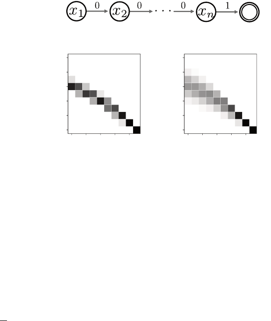
More often than not, however, the random returns are not normally distributed.

This may be because the rewards themselves are not normally distributed, or

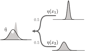
because the transition kernel is stochastic. Figure 5.1 illustrates the eﬀect of

the distributional Bellman operator on a normal return-distribution function

mixing the return distributions at successor states results in a mixture of normal

distributions, which is not normally distributed except in trivial situations. In

other words, the normal representation

is generally not closed under the

distributional Bellman operator.

Rather than represent the return distribution with high accuracy, as with the

empirical distribution, let us consider the more modest goal of determining the

best normal approximation to the return-distribution function

. We deﬁne

“best normal approximation” as

ˆη

(x) = N



(x), Var



(x)





. (5.16)

Given that a normal distribution is parameterized by its mean and variance, this

is an obviously sensible choice. In some cases, this choice can also be justiﬁed

by arguing that

ˆη

(

) is the normal distribution closest to

(

) in terms of what

is called the Kullback–Leibler divergence.

As we now show, this choice also

leads to a particularly eﬃcient algorithm for computing ˆη

We will construct an iterative procedure that operates on return functions

from a normal representation and converges to

ˆη

. We start with the random

variable operator





(x)

= R + γG(X

), X = x , (5.17)

39.

Technically, this is only true when the return distribution

(

) has a probability density function.

When

(

) does not have a density, a similar argument can be made in terms with the cross-entropy

loss; see Exercises 5.5 and 5.6.

Draft version.

126 Chapter 5

Return

Figure 5.1

Applying the distributional Bellman oper-

ator to a return function

described by the

normal representation generally produces

return distributions that are not normally

distributed. Here, a uniform mixture of two

normal distributions (shown as probability

densities) results in a bimodal distribution

(in light gray). The best normal approxi-

mation

ˆη

to that distribution is depicted by

the solid curve.

and take expectations on both sides of the equation:



G)(x)



= E

R + γE[G(X

) | X

] | X = x

= E

[R | X = x] + γ E

[E[G(X

) | X

] | X = x]

= E

[R | X = x] + γ

∈X

= x

| X = x) E[G(x

)] , (5.18)

where the last step follows from the assumption that the random variables

are

independent of the next-state

. When applied to the return-variable function

, Equation 5.18 is none other than the classical Bellman equation.

The same technique allows us to relate the variance of (

)(

) to the

next-state variances. For a random variable Z, recall that

Var(Z) = E



(Z −E[Z])



The random reward

and next-state

are by deﬁnition conditionally indepen-

dent given

and

. However, to simplify the exposition, we assume that they

are also conditionally independent given only

(in Chapter 8, we will see how

this assumption can be avoided).

Let us use the notation

Var

to make explicit the dependency of certain

random variables on the sample transition model, analogous to our use of

Denote the value function corresponding to G by V(x) = E[G(x)]. We have

Var



G)(x)



= Var



R + γG(X

) | X = x



= Var



R | X = x



+ Var



γG(X

) | X = x



= Var



R | X = x



+ γ

Var



G(X

) | X = x



= Var



R | X = x



+ γ

Var



V(X

) | X = x



40.

In Equation 5.18, some of the expectations are taken solely with respect to the sample transition

model, which we denote by

as usual. The expectation with respect to the random variable

, on

the other hand, is not part of the model; we use the unsubscripted E to emphasize this point.

Draft version.

Distributional Dynamic Programming 127

+ γ

∈X

= x

| X = x)Var



G(x

)



, (5.19)

where the last line follows by the law of total variance:

Var(A) = Var



E[A | B]



+ E



Var[A | B]



Equation 5.19 shows how to compute the variances of the return function

Speciﬁcally, these variances depend on the reward variance, the variance in

next-state values, and the expected next-state variances. When

, this is

the Bellman equation for the variance of the random return. Writing

(

) =

Var



(x)



, we obtain

(x) = Var

(R | X = x) + γ

Var



) | X = x



+ γ

∈X

= x

| X = x)σ

(x) . (5.20)

We now combine the results above to obtain a dynamic programming proce-

dure for ﬁnding

ˆη

. For each state

x ∈X

, let us denote by

(

) and

(

) the

parameters of a return-distribution distribution

with

(

) =



(

)

, σ

(

)



For all x, we simultaneously compute

k+1

(x) = E

[R + γµ

) | X = x] (5.21)

k+1

(x) = Var



R | X = x



+ γ

Var



) | X = x



+ γ

[σ

) | X = x] .

(5.22)

We can view these two updates as the implementation of a bona ﬁde operator

over the space of normal return-distribution functions. Indeed, we can associate

to each iteration the return function

(x) = N



(x), σ

(x)



∈F

Analyzing the behavior of the sequence (

)

k≥0

require some care, but we

shall see in Chapter 8 that the iterates converge to the best approximation

ˆη

(Equation 5.16), in the sense that for all x ∈X,

(x) →V

(x) σ

(x) →Var



(x)



This derivation shows that the normal representation can be used to create a

tractable algorithm for approximating the return distribution. However, in our

work, we have found that the normal representation rarely gives a satisfying

depiction of the agent’s interactions with its environment; it is not suﬃciently

expressive. In many problems, outcomes are discrete in nature: success or

failure, food or hunger, forward motion or fall. This arises in video games in

which the game ends once the player’s last life is spent. Timing is also critical:

to catch the diamond, key, or mushroom, the agent must press “jump” at just the

Draft version.

128 Chapter 5

right moment, again leading to discrete outcomes. Even in relatively continuous

systems, such as the application of reinforcement learning to stratospheric

balloon ﬂight, the return distributions tend to be skewed or multimodal. In short,

normal distributions are a poor ﬁt for the wide gamut of problems found in

reinforcement learning.

5.5 Fixed-Size Empirical Representations

The empirical representation is expressive because it can use more particles to

describe more complex probability distributions. This “blank check” approach

to memory and computation, however, results in an intractable algorithm. On

the other hand, the simple normal distribution is rarely suﬃcient to give a

good approximation of the return distribution. A good middle ground is to

preserve the form of the empirical representation while imposing a limit on its

expressivity. Our approach is to ﬁx the number and type of particles used to

represent probability distributions.

Deﬁnition 5.11.

The

-quantile representation parameterizes the location of

m equally weighted particles. That is,

Q,m

(

i=1

: θ

∈R

)

. 4

Deﬁnition 5.12.

Given a collection of

evenly spaced locations

< ···< θ

the

-categorical representation parameterizes the probability of

particles at

these ﬁxed locations:

C,m

(

i=1

: p

≥0,

i=1

= 1

)

We denote the stride between successive particles by ς

−θ

m−1

. 4

This deﬁnition corresponds to the categorical representation used in Chapter

3. Note that because of the constraint that probabilities should sum to 1, a

categorical distribution is described by

m −

1 parameters. In addition, although

the representation depends on the choice of locations

, …, θ

, we omit this

dependence in the notation F

C,m

to keep things concise.

In our deﬁnition of the

-categorical representation, we assume that the

locations (

)

i=1

are given a priori and not part of the description of a particular

probability distribution. This is sensible when we consider that algorithms such

as categorical temporal-diﬀerence learning use the same set of locations to

describe distributions at diﬀerent states and keep these locations ﬁxed across

the learning process. For example, a common choice is

min

and

max

Draft version.

Distributional Dynamic Programming 129

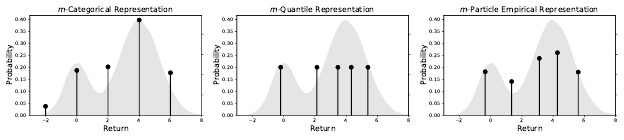
Figure 5.2

A distribution

(in light gray), as approximated with a

-categorical,

-quantile, or

m-particle representation, for m = 5.

When it is desirable to adjust both the locations and probabilities of diﬀerent

particles, we instead make use of the m-particle representation.

Deﬁnition 5.13.

The

-particle representation parameterizes both the proba-

bility and location of m particles:

E,m

(

i=1

: θ

∈R, p

≥0,

i=1

= 1

)

The

-particle representation contains both the

-quantile representation and

the

-categorical representation; a distribution from

E,m

is deﬁned by 2

m −

parameters. 4

Mathematically, all three representations described above are subsets of

the empirical representation

; accordingly, we call them ﬁxed-size empiri-

cal representations. Fixed-size empirical representations are ﬂexible and can

approximate both continuous and discrete outcome distributions (Figure 5.2).

The categorical representation is so called because it models the probability

of a set of ﬁxed outcomes. This is somewhat of a misnomer: the “categories”

are not arbitrary but instead correspond to speciﬁc real values. The quantile

representation is named for its relationship to the quantiles of the return distri-

bution. Although it might seem like the

-particle representation is a strictly

superior choice, we will see that committing to either ﬁxed locations or ﬁxed

probabilities simpliﬁes algorithmic design. For an equal number of parameters,

it is also not clear whether one should prefer

fully parameterized particles or,

say, 2m −1 uniformly weighted particles.

Like the normal representation, ﬁxed-size empirical representations are not

closed under the distributional Bellman operator

. As discussed in Section

5.3, the consequence is that we cannot implement the iterative procedure

k+1

= T

Draft version.

130 Chapter 5

with such a representation. To get around this issue, let us now introduce

the notion of a projection operator: a mapping from the space of probability

distributions (or a subset thereof) to a desired representation

We denote

such an operator by

: P(R) →F .

Deﬁnitionally, we require that projection operators satisfy, for any ν ∈F ,

ν = ν .

We extend the notation Π

to the space of return-distribution functions:





(x) = Π



η(x)



The categorical projection Π

, ﬁrst encountered in Chapter 3, is one such

operator; we will study it in greater detail in the remainder of this chapter.

We also made implicit use of a projection step in deriving an algorithm for

the normal representation: at each iteration, we kept track of the mean and

variance of the process but discarded the rest of the distribution, so that the

return function iterates could be described with the normal representation.

Algorithmically, we introduce a projection step following the application of

, leading to a projected distributional Bellman operator Π

. By deﬁni-

tion, this operator maps

to itself, allowing for the design of distributional

algorithms that represent each iterate of the sequence

k+1

= Π

using a bounded amount of memory. We will discuss such algorithmic con-

siderations in Section 5.7, after describing particular projection operators for

the categorical and quantile representations. Combined with numerical integra-

tion, the use of a projection step also makes it possible to perform dynamic

programming with continuous reward distributions (see Exercise 5.9).

5.6 The Projection Step

We now describe projection operators for the categorical and quantile represen-

tations, correspondingly called categorical projection and quantile projection.

In both cases, these operators can be seen as ﬁnding the best approximation to a

given probability distribution, as measured according to a speciﬁc probability

metric.

To begin, recall that for a probability metric

(

)

⊆P

(

) is the set of

probability distributions with ﬁnite mean and ﬁnite distance from the reference

41.

In Section 4.1, we deﬁned an operator as mapping elements from a space to itself. The term

“projection operator” here is reasonable given that F ⊆P(R).

Draft version.

Distributional Dynamic Programming 131

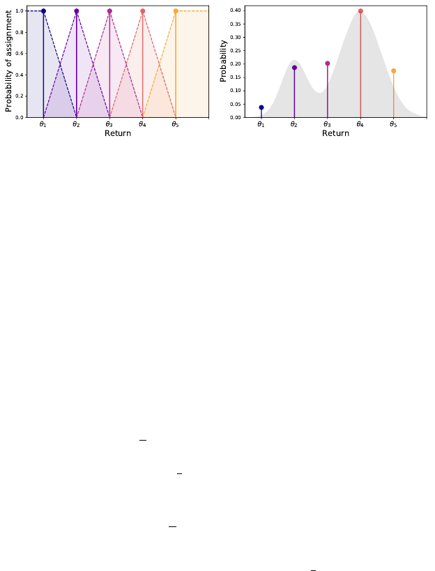
Figure 5.3

Left

: The categorical projection assigns probability mass to each location according to

a triangular kernel (central locations) and half-triangular kernels (boundary locations).

Here,

= 5.

Right

: The

= 5 categorical projection of a given distribution, shown in

gray. Each Dirac delta is colored to match its kernel in the left panel.

distribution

(Equation 4.26). For a representation

F ⊆P

(

), a

-projection

ν ∈P

(

) onto

is a function Π

F ,d

(

)

→F

that ﬁnds a distribution

ˆν ∈F that is d-closest to ν:

F ,d

ν ∈arg min

ˆν∈F

d(ν, ˆν) . (5.23)

Although both the categorical and quantile projections that we present here

satisfy this deﬁnition, it is worth noting that in the most general setting, neither

the existence nor uniqueness of a

-projection Π

F ,d

is actually guaranteed (see

Remark 5.3). We lift the notion of a

-projection to return-distribution functions

in our usual manner; the d-projection of η ∈P

(R)

onto F





(x) = Π

F ,d



η(x)



When unambiguous, we overload notation and write Π

F ,d

to denote the

projection onto F

It is natural to think of the

-projection of the return-distribution function

onto

as the best achievable approximation within this representation,

measured in terms of

. We thus call Π

F ,d

and Π

the (

d, F

)-optimal

approximations to ν ∈P(R) and η, respectively.

Categorical projection.

In Chapter 3, we deﬁned the categorical projection

as assigning the probability mass

of a particle located at

to the two loca-

tions nearest to

in the ﬁxed support

{θ

, . . . , θ

}

. Speciﬁcally, the categorical

projection assigns this mass

in (inverse) proportion to the distance to these

two neighbors. We now extend this idea to the case where we wish to more

generally project a distribution

ν ∈P

(

) onto the

-categorical representation.

Draft version.

132 Chapter 5

Given a probability distribution ν ∈P

(R), its categorical projection

ν =

i=1

has parameters

= E

Z∼ν



−1



Z −θ



i

, i = 1, . . . , m , (5.24)

for a set of functions

R →

1] that we will deﬁne below. Here we write

in terms of an expectation rather than a sum, with the idea that this expectation

can be eﬃciently computed (this is the case when

is itself a

-categorical

distribution).

When i = 2, . . . , m −1, the function h

is the triangular kernel

(z) = h(z) = max(0, 1 −|z|) .

We use this notation to describe the proportional assignment of probability mass

for the inner locations

, . . . , θ

m−1

. One can verify that the triangular kernel

assigns probability mass from

to the location

in proportion to the distance

to its neighbors (Figure 5.3).

The parameters of the extreme locations are computed somewhat diﬀerently,

as these also capture the probability mass associated with values greater than

and smaller than θ

. For these, we use the half-triangular kernels

(z) =

(

1 z ≤0

max(0, 1 −|z|) z > 0

(z) =

(

max(0, 1 −|z|) z ≤0

1 z > 0 .

Exercise 5.10 asks you to prove that the projection described here matches to

deterministic projection of Section 3.5.

Our derivation gives a mathematical formalization of the idea of assign-

ing proportional probability mass to the locations nearest to a given particle,

described in Chapter 3. In fact, it also describes the projection of

in the Cramér

distance (



) onto the

-categorical representation. This is stated formally as

follows and proven in Remark 5.4.

Proposition 5.14.

Let

ν ∈P

(

). The

-categorical probability distri-

bution whose parameters are given by Equation 5.24 is the (unique)



-projection onto F

C,m

. 4

Quantile projection.

We call the quantile projection of a probability dis-

tribution of

ν ∈P

(

) a speciﬁc projection of

in the 1-Wasserstein distance

(

) onto the

-quantile representation (Π

Q,m

). With this choice of distance,

this projection can be expressed in closed form and is easily implemented. In

addition, we will see in Section 5.9 that it leads to a well-behaved dynamic

Draft version.

Distributional Dynamic Programming 133

programming algorithm. As with the categorical projection, we introduce the

shorthand Π

for the projection operator Π

Q,m

Consider a probability distribution

ν ∈P

(

). We are interested in a proba-

bility distribution Π

ν ∈F

Q,m

that minimizes the 1-Wasserstein distance from

ν:

minimize w

(ν, ν

) subject to ν

∈F

Q,m

By deﬁnition, such a solution must take the form

ν =

i=1

The following establishes that choosing (

)

i=1

to be a particular set of quantiles

of ν yields a valid w

-projection of ν.

Proposition 5.15.

Let

ν ∈P

(

). The

-quantile probability distribution

whose parameters are given by

= F

−1

2i −1

i = 1, . . . , m (5.25)

is a w

-projection of ν onto F

Q,m

. 4

Equation 5.25 arises because the

th particle of a

-quantile distribution is

“responsible” for the portion of the 1-Wasserstein distance measured on the

interval [

i−1

] (Figure 5.4). As formalized by the following lemma, the choice

of the midpoint quantile

2i−1

minimizes the 1-Wasserstein distance to

on this

interval.

Lemma 5.16.

Let

ν ∈P

(

) with cumulative distribution function

. Let

0 ≤a < b ≤1. Then a solution to

min

θ∈R



−1

(τ) −θ



dτ (5.26)

is given by the quantile midpoint

θ = F

−1

a + b

. 4

The proof is given as Remark 5.5.

Proof of Proposition 5.15.

Let

i=1

be a

-quantile distribution.

Assume that its locations are sorted: that is,

≤θ

≤···≤θ

. For

τ ∈

1),

its inverse cumulative distribution function is

−1

(τ) = θ

dτme

Draft version.

134 Chapter 5

2 0 2 4 6 8

Return

0.0

0.2

0.4

0.6

0.8

1.0

Cumulative Probability

2 0 2 4 6 8

Return

0.0

0.1

0.2

0.3

0.4

Probability

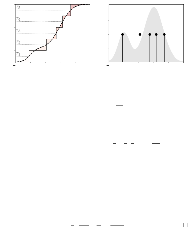
Figure 5.4

Left

: The quantile projection ﬁnds the quantiles of the distribution

(the dashed line

depicts its cumulative distribution function) for

2i−1

, i

= 1

, . . . m

. The shaded area

corresponds to the 1-Wasserstein distance between

and its quantile projection Π

(solid line,

= 5).

Right

: The optimal (

, F

Q,m

)-approximation to the distribution

shown in gray.

This function is constant on the intervals (0

)

[

)

, . . . ,

[

m−1

1). The 1-

Wasserstein distance between

and

therefore decomposes into a sum of

terms:

(ν, ν

) =



−1

(τ) − F

−1

(τ)



dτ

i=1

(i−1)



−1

(τ) −θ



dτ .

By Lemma 5.16, the

th term of the sum is minimized by the quantile midpoint

−1

(τ

), where

i −1

2i −1

Unlike the categorical-Cramér case, in general, there is not a unique

quantile distribution

∈F

Q,m

that is closest in

to a given distribution

ν ∈

(R). The following example illustrates how the issue might take shape.

Example 5.17. Consider the set of Dirac distributions

Q,1

= {δ

: θ ∈R}.

Draft version.

Distributional Dynamic Programming 135

Let

be the Bernoulli(

) distribution. For any

θ ∈

1],

∈F

Q,1

is an optimal (w

, F

Q,1

)-approximation to ν:

(ν, δ

) = min

∈F

Q,1

(ν, ν

) ,

Perhaps surprisingly, this shows that the distribution

, halfway between the

two possible outcomes and an intuitive one-particle approximation to

, is a no

better choice than δ

when measured in terms of 1-Wasserstein distance. 4

5.7 Distributional Dynamic Programming

We embed the projected Bellman operator in an

for

loop to obtain an algorithmic

template for approximating the return function (Algorithm 5.2). We call this

template distributional dynamic programming (DDP),

as it computes

k+1

= Π

(5.27)

by iteratively applying a projected distributional Bellman operator. A special

case is when the representation is closed under

, in which case no projection

is needed. However, by contrast with Equation 5.6, the use of a projection allows

us to consider algorithms for a greater variety of representations. Summarizing

the results of the previous sections, instantiating this template involves three

parts:

Choice of representation. We ﬁrst need a probability distribution represen-

tation

. Provided that this representation uses ﬁnitely many parameters, this

enables us to store return functions in memory, using the implied mapping from

parameters to probability distributions.

Update step.

We then need a subroutine for computing a single application

of the distributional Bellman operator to a return function represented by

(Equation 5.8).

Projection step.

We ﬁnally need a subroutine that maps the outputs of the

update step to probability distributions in

. In particular, when Π

is a

-projection, this involves ﬁnding an optimal (

d, F

)-approximation at each

iteration.

For empirical representations, including the categorical and quantile repre-

sentations, the update step can be implemented by Algorithm 5.1. That is, when

there are ﬁnitely many rewards, the output of

applied to any

-particle

representation is a collection of empirical distributions:

η ∈F

E,m

=⇒ T

η ∈F

42.

More precisely, this is distributional dynamic programming applied to the problem of policy

evaluation. A sensible but less memorable alternative is “iterative distributional policy evaluation.”

Draft version.

136 Chapter 5

Algorithm 5.2: Distributional dynamic programming

Algorithm parameters: representation F , projection Π

desired number of iterations K,

initial return function η

∈F

Initialize η ←η

for k = 1, . . . , K do

←T

η  Algorithm 5.1

foreach state x ∈X do

η(x) ←(Π

)(x)

end foreach

end for

return η

As a consequence, it is suﬃcient to have an eﬃcient subroutine for projecting

empirical distributions back to F

C,m

, F

Q,m

, or F

E,m

For example, consider the projection of the empirical distribution

ν =

j=1

onto the

-categorical representation (Deﬁnition 5.12). For

= 1

, . . . , m

Equation 5.24 becomes

j=1



−1

−θ

)



which can be implemented in linear time with two for loops (as was done in

Algorithm 3.4).

Similarly, the projection of

onto the

-quantile representation (Deﬁni-

tion 5.11) is achieved by sorting the locations

to construct the cumulative

distribution function from their associated probabilities q

(z) =

j=1

j {z

≤z}

from which quantile midpoints can be extracted.

Because the categorical-Cramér and quantile-

pairs recur so often through-

out this book, it is convenient to give a name to the algorithms that iteratively

apply their respective projected operators. We call these algorithms categorical

Draft version.

Distributional Dynamic Programming 137

Algorithm 5.3: Categorical dynamic programming

Algorithm parameters: representation parameters θ

, . . . , θ

, m,

initial probabilities



(x))

i=1

: x ∈X



desired number of iterations K

for k = 1, . . . , K do

η(x) =

i=1

(x)δ

for x ∈X



(x), p

(x)



m(x)

j=1

: x ∈X



←T

η  Algorithm 5.1

foreach state x ∈X do

for i = 1, …, m do

(x) ←

m(x)

j=1

(x)h



−1

−θ

)



end for

end foreach

end for

return



(x))

i=1

: x ∈X)

and quantile dynamic programming, respectively (CDP and QDP; Algorithms

5.3 and 5.4).

For both categorical and quantile dynamic programming, the computational

cost is dominated by the number of particles produced by the distributional

Bellman operator, prior to projection. Since the number of particles in the

representation is a constant

, we have that per state, there may be up to

particles in this intermediate step. Thus, the cost of

iterations

with the

-categorical representation is

(

KmN

), not too dissimilar to the

cost of performing iterative policy evaluation with value functions. Due to the

sorting operation, the cost of

iterations with the

-quantile representation is

larger, at



KmN

log

(

)



. In Chapter 6, we describe an incremental

algorithm that avoids the explicit sorting operation and is in some cases more

computationally eﬃcient.

In designing distributional dynamic programming algorithms, there is a good

deal of ﬂexibility in the choice of representation and in the projection step once

a representation has been selected. There are basic properties we would like

43.

To be fully accurate, we should call these the categorical-Cramér and quantile-

dynamic

programming algorithms, given that they combine particular choices of probability representation

and projection. However, brevity has its virtues.

Draft version.

138 Chapter 5

Algorithm 5.4: Quantile dynamic programming

Algorithm parameters: initial locations



(θ

(x))

i=1

: x ∈X),

desired number of iterations K

for k = 1, . . . , K do

η(x) =

i=1

(x)

for x ∈X



(x), p

(x)



m(x)

j=1

: x ∈X



←T

η  Algorithm 5.1

foreach state x ∈X do

(x), p

(x))

m(x)

i=1

←sort ((z

(x), p

(x))

m(x)

i=1

)

for j = 1, …, m do

(x) ←

i=1

(x)

end for

for i = 1, …, m do

j ←min{l : P

(x) ≥τ

}

(x) ←z

(x)

end for

end foreach

end for

return



(θ

(x))

i=1

: x ∈X



from the sequence deﬁned by Equation 5.27, such as a guarantee of convergence,

and further a limit that does not depend on our choice of initialization. Certain

combinations of representation and projection will ensure these properties hold,

as we explore in Section 5.9, while others may lead to very poorly behaved

algorithms (see Exercise 5.19). In addition, using a representation and projection

also necessarily incurs some approximation error relative to the true return

function. It is often possible to obtain quantitative bounds on this approximation

error, as Section 5.10 describes, but often judgment must be used as to what

qualitative types of approximation are the most acceptable for task in hand; we

return to this point in Section 5.11.

5.8 Error Due to Diﬀusion

In Section 5.4, we showed that the distributional algorithm for the normal

representation ﬁnds the best ﬁt to the return function

, as measured in

Kullback–Leibler divergence. Implicit in our derivation was the fact that we

Draft version.

Distributional Dynamic Programming 139

··· η

ˆη

··· ˆη

Figure 5.5

A diﬀusion-free projection operator Π

yields a distributional dynamic program-

ming procedure that is equivalent to ﬁrst computing an exact return function and then

projecting it.

could interleave projection and update steps to obtain the same solution as if

we had ﬁrst determined

without approximation and then found its best ﬁt in

. We call a projection operator with this property diﬀusion-free (Figure 5.5).

Deﬁnition 5.18.

Consider a representation

and a projection operator Π

for that representation. The projection operator Π

is said to be diﬀusion-free

if, for any return function η ∈F

, we have

η = Π

η .

As a consequence, for any

k ≥

0 and any

η ∈F

, a diﬀusion-free projection

operator satisﬁes

(Π

)

η = Π

)

η . 4

Algorithms that implement diﬀusion-free projection operators are quite

appealing, because they behave as if no approximation had been made until the

ﬁnal iteration. Unfortunately, such algorithms are the exception, rather than the

rule. By contrast, without this guarantee, an algorithm may accumulate excess

error from iteration to iteration – we say that the iterates

, η

, . . .

undergo

diﬀusion. Known projection algorithms for

-particle representations suﬀer

from this issue, as the following example illustrates.

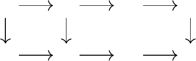
Example 5.19.

Consider a chain of

states with a deterministic left-to-right

transition function (Figure 5.6). The last state of this chain, x

, is terminal and

produces a reward of 1; all other states yield no reward. For

t ≥

0, the discounted

return at state

n−t

is deterministic and has value

; let us denote its distribution

(

n−t

). If we approximate this distribution with

= 11 particles uniformly

spaced from 0 to 1, the best categorical approximation assigns probability to

the two particles closest to γ

If we instead use categorical dynamic programming, we ﬁnd a diﬀerent

solution. Because each iteration of the projected Bellman operator must produce

Draft version.

140 Chapter 5

State

Return

m-Categorical

Approximation

0.0

0.2

0.4

0.6

0.8

1.0

State

Return

Categorical

Dynamic Programming

0.0

0.2

0.4

0.6

0.8

1.0

(a)

(b) (c)

Figure 5.6

(a)

-state chain with a single nonzero reward at the end.

(b)

The (



, F

C,m

)-optimal

approximation to the return function, for

= 10,

= 11, and

= 0

, . . . , θ

= 1. The

probabilities assigned to each location are indicated in grayscale (white = 0, black =

1).

(c)

The approximation found by categorical dynamic programming with the same

representation.

a categorical distribution, the iterates undergo diﬀusion. Far from the terminal

state, the return distribution found by Algorithm 5.2 is distributed on a much

larger support than the best categorical approximation of η(x

). 4

The diﬀusion in Example 5.19 can be explained analytically. Let us asso-

ciate each particle with an integer

= 0

, . . . ,

10, corresponding to the location

. For concreteness, let

= 1

−ε

for some 0

< ε 

1, and consider the

return-distribution function obtained after

iterations of categorical dynamic

programming:

ˆη = (Π

)

Because there are no cycles, one can show that further iterations leave the

approximation unchanged.

If we interpret the

particle locations as states in a Markov chain, then we

can view the return distribution

ˆη

(

n−t

) as the probability distribution of this

Markov chain after

time steps (

t ∈{

, . . . , n −

}

). The transition function for

states j = 1 . . . 10 is

P(bγ jc | j) = dγ je−γ j

P(dγ je | j) = 1 −dγ je+ γ j .

For

= 0, we simply have

0) = 1 (i.e., state 0 is terminal). When

suﬃciently small compared to the gap

= 0

1 between neighboring particle

Draft version.

Distributional Dynamic Programming 141

locations, the process can be approximated with a binomial distribution:

G(x

n−t

) ∼1 −t

−1

Binom(1 −γ, t) ,

where

is the return-variable function associated with

ˆη

. Figure 5.6c gives a

rough illustration of this point, with a bell-shaped distribution emerging in the

return distribution at state x

5.9 Convergence of Distributional Dynamic Programming

We now use the theory of operators developed in Chapter 4 to characterize the

behavior of distributional dynamic programming in the policy evaluation setting:

its convergence rate, its point of convergence, and also the approximation error

incurred. Speciﬁcally, this theory allows us to measure how these quantities

are impacted by diﬀerent choices of representation and projection. Although

the algorithmic discussion in previous sections has focused on implementa-

tions of distributional dynamic programming in the case of ﬁnitely supported

reward distributions, the results presented here apply without this assumption

(see Exercise 5.9 for indications of how distributional dynamic programming

algorithms may be implemented in such cases). As we will see in Chapter 6,

the theory developed here also informs incremental algorithms for learning the

return-distribution function.

Let us consider a probability metric

, possibly diﬀerent from the metric

under which the projection is performed (when applicable), and which we call

the analysis metric. We use the analysis metric to characterize instances of

Algorithm 5.2 in terms of the Lipschitz constant of the projected operator.

Deﬁnition 5.20.

Let (

M, d

) be a metric space, and let

M → M

be a function

on this space. The Lipschitz constant of O under the metric d is

kOk

= sup

U,U

∈M

U,U

d(OU, OU

)

d(U, U

)

. 4

When

is a contraction mapping, its Lipschitz constant is simply its con-

traction modulus. That is, under the conditions of Theorem 4.25 applied to a

c-homogeneous d, we have

≤γ

Deﬁnition 5.20 extends the notion of a contraction modulus to operators, such

as projections, that are not contraction mappings.

Lemma 5.21.

Let (

M, d

) be a metric space, and let

, O

M → M

be func-

tions on this space. Write

for the composition of these mappings.

Then,

≤kO

. 4

Draft version.

142 Chapter 5

Proof. By applying the deﬁnition of the Lipschitz constant twice, we have

d(O

U, O

) ≤kO

d(O

U, O

) ≤kO

d(U, U

) ,

as required.

Lemma 5.21 gives a template for validating and understanding diﬀerent

instantiations of Algorithm 5.2. Here, we consider the metric space deﬁned by

the ﬁnite domain of our analysis metric, (

(

)

, d

), and use Lemma 5.21 to

characterize Π

in terms of the Lipschitz constants of its parts (Π

and

). By analogy with the conditions of Proposition 4.27, where needed, we

will assume that the environment (more speciﬁcally, its random quantities) is

reasonably behaved under d.

Assumption 5.22(d).

The ﬁnite domain

(

)

is closed under both the

projection Π

and the Bellman operator T

, in the sense that

η ∈P

(R)

=⇒ T

η, Π

η ∈P

(R)

. 4

Assumption 5.22(

) guarantees that distributions produced by the distri-

butional Bellman operator and the projection have ﬁnite distances from one

another. For many choices of

of interest, Assumption 5.22 can be easily shown

to hold when the reward distributions are bounded; contrast with Proposition

4.16.

The Lipschitz constant of projection operators must be at least 1, since for

any ν ∈F ,

ν = ν .

In the case of the Cramér distance 

, we can show that it behaves much like a

Euclidean metric, from which we obtain the following result on



projections.

Lemma 5.23.

Consider a representation

F ⊆P



(

). If

is complete with

respect to



and convex, then the



-projection Π

F ,



(

)

→F

is a

nonexpansion in that metric:

kΠ

F ,



= 1 .

Furthermore, the result extends to return functions and the supremum extension

of 

kΠ

F ,



= 1 . 4

The proof is given in Remark 5.6. Exercise 5.15 asks you show that the

-categorical representation is convex and complete with respect to the Cramér

distance. From this, we immediately derive the following.

Lemma 5.24.

The projected distributional Bellman operator instantiated with

C,m

and



has contraction modulus

with respect to



on the

Draft version.

Distributional Dynamic Programming 143

space P



(R)

. That is,

kΠ



≤γ

. 4

Lemma 5.24 gives a formal reason for why the use of the

-categorical

representation, coupled with a projection based on triangular kernel, produces a

convergent distributional dynamic programming algorithm.

The

-quantile representation, however, is not convex. This precludes a direct

appeal to an argument based on a quantile analogue to Lemma 5.23. Nor is

the issue simply analytical: the

Lipschitz constant of the projected Bellman

operator Π

is greater than 1 (see Exercise 5.16). Instead, we need to use the

∞

-Wasserstein distance as our analysis metric. As the

-projection onto

Q,m

is a nonexpansion in w

∞

, we obtain the following result.

Lemma 5.25.

Under Assumption 5.22(

∞

), the projected distributional Bell-

man operator Π

∞

(

)

→P

∞

(

)

has contraction modulus

∞

That is,

kΠ

∞

≤γ . 4

Proof.

Since

is a

-contraction in

∞

by Proposition 4.15, it is suﬃcient

to prove that Π

∞

(

)

→P

∞

(

) is a nonexpansion in

∞

; the result then

follows from Lemma 5.21. Given two distributions ν

, ν

∈P

∞

(R), we have

∞

(ν

, ν

) = sup

τ∈(0,1)

−1

(τ) −F

−1

(τ)|.

Now note that

i=1

−1

(τ

)

, Π

i=1

−1

(τ

)

where τ

2i−1

. We have

∞

(Π

, Π

) = max

i=1,…,m



−1

(τ

) −F

−1

(τ

)



≤ sup

τ∈(0,1)



−1

(τ) −F

−1

(τ)



= w

∞

(ν

, ν

) ,

as required.

The derivation of a contraction modulus for a projected Bellman operator

provides us with two results. By Proposition 4.7, it establishes that if Π

has a ﬁxed point

ˆη

, then Algorithm 5.2 converges to this ﬁxed point. Second, it

also establishes the existence of such a ﬁxed point when the representation is

complete with respect to the analysis metric

, based on Banach’s ﬁxed point

theorem; a proof is provided in Remark 5.7.

Draft version.

144 Chapter 5

Theorem 5.26

(Banach’s ﬁxed point theorem)

Let (

M, d

) be a complete

metric space and let

be a contraction mapping on

, with respect to

Then O has a unique ﬁxed point U

∗

∈ M. 4

Proposition 5.27.

Let

be a

-homogeneous, regular probability metric

that is

-convex for some

p ∈

, ∞

) and let

be a representation complete

with respect to

. Consider Algorithm 5.2 instantiated with a projection

step described by the operator Π

, and suppose that Assumption 5.22(

)

holds. If Π

is a nonexpansion in

, then the corresponding projected

Bellman operator Π

has a unique ﬁxed point

ˆη

(

)

satisfying

ˆη

= Π

ˆη

Additionally, for any ε > 0, if K the number of iterations is such that

K ≥

log





+ log d(η

, ˆη

)

c log





with

(

)

∈P

(

) for all

, then the output

of Algorithm 5.2 satisﬁes

d(η

, ˆη

) ≤ε . 4

Proof.

By the assumptions in the statement, we have that

is a

-contraction

(

)

by Theorem 4.25, and by Lemma 5.21, Π

is a

-contraction

(

)

. By Banach’s ﬁxed point theorem, there is a unique ﬁxed point

ˆη

for Π

in P

(R)

. Now note

d(η

, ˆη

) = d(Π

K−1

, Π

ˆη

) ≤γ

d(η

K−1

, ˆη

) ,

so by induction

d(η

, ˆη

) ≤γ

d(η

, ˆη

) .

Setting the right-hand side to less than

and rearranging yields the result.

Although Proposition 5.27 does not allow us to conclude that a particular

algorithm will fail, it cautions us against projections in certain probability

metrics. For example, because the distributional Bellman operator is only a non-

expansion in the supremum total variation distance, we cannot guarantee a good

approximation with respect to this metric after any ﬁnite number of iterations.

Because we would like the projection step to be computationally eﬃcient, this

argument also gives us a criterion with which to choose a representation. For

example, although the

-particle representation is clearly more ﬂexible than

Draft version.

Distributional Dynamic Programming 145

either the categorical or quantile representations, it is currently not known how

to eﬃciently and usefully project onto it.

5.10 Quality of the Distributional Approximation

Having identiﬁed conditions under which the iterates produced by distributional

dynamic programming converge, we now ask: to what do they converge? We

answer this question by measuring how close the ﬁxed point

ˆη

of the projected

Bellman operator (computed by Algorithm 5.2 in the limit of the number of

iterations) is to the true return function

. The quality of this approximation

depends on a number of factors: the choice and size of representation

, which

determines the optimal approximation of

within

, as well as properties of

the projection step.

Proposition 5.28.

Let

be a

-homogeneous, regular probability metric

that is

-convex for some

p ∈

, ∞

), and let

F ⊆P

(

) be a representation

complete with respect to

. Let Π

be a projection operator that is a

nonexpansion in

, and suppose Assumption 5.22(

) holds. Consider the

projected Bellman operator Π

with ﬁxed point ˆη

∈P

(R)

. Then,

d(ˆη

, η

) ≤

d(Π

, η

)

1 −γ

When Π

is a

-projection in some probability metric

, Π

is a

(d, F )-optimal approximation of the return function η

. 4

Proof. We have

d(η

, ˆη

) ≤d(η

, Π

) + d(Π

, ˆη

)

= d (η

, Π

) + d(Π

, Π

ˆη

)

≤d (η

, Π

) + γ

d(η

, ˆη

) .

Rearranging then gives the result.

From this, we immediately derive a result regarding the ﬁxed point

ˆη

of the

projected operator Π

Corollary 5.29.

The ﬁxed point

ˆη

of the categorical-projected Bellman

operator Π

: P

(R) →P

(R) satisﬁes



(ˆη

, η

) ≤



(Π

, η

)

1 −γ

Draft version.

146 Chapter 5

Figure 5.7

The return-distribution function estimates obtained by applying categorical dynamic

programming to the Cliﬀs domain (Example 2.9; here, with the safe policy). Each panel

corresponds to a diﬀerent number of particles.

If the return distributions (

(

) :

x ∈X

) are supported on [

, θ

], we further

have that, for each x ∈X,

min

ν∈F

C,m



(ν, η

(x)) ≤ς

i=1



(x)



+ iς



−F

(x)



+ (i −1)ς





≤ς

(5.28)

and hence



(ˆη

, η

) ≤

1 −γ

−θ

m −1

. 4

Proposition 5.28 suggests that the excess error may be greater when the

projection is performed in a metric for which

is small. In the particular case of

the Cramér distance, the constant in Corollary 5.29 can in fact be strengthened

√

1−γ

by arguing about the geometry of the probability space under



under certain conditions; see Remark 5.6 for a discussion of this geometry and

Rowland et al. (2018) for details on the strengthened bound.

Varying the number of particles in the categorical representation allows the

user to control both the complexity of the associated dynamic programming

algorithm and the error of the ﬁxed point

ˆη

(Figure 5.7). As discussed in the

ﬁrst part of this chapter, both the memory and time complexity of computing

with this representation increase with

. On the other hand, Corollary 5.29

establishes that increasing

also reduces the approximation error incurred from

dynamic programming.

Proposition 5.28 can be similarly used to analyze quantile dynamic pro-

gramming. This result, under the conditions of Lemma 5.25, shows that the

ﬁxed point

ˆη

of the projected operator Π

for the

-quantile representation

satisﬁes

∞

(ˆη

, η

) ≤

∞

(Π

, η

)

1 −γ

Draft version.

Distributional Dynamic Programming 147

Unfortunately, the distance

∞

(Π

, η

) does not necessarily vanish as the

number of particles

in the quantile representation increases. This is because

∞

is in some sense a very strict distance (Exercise 5.18 makes this point

precise). Nevertheless, the dynamic programming algorithm associated with the

quantile representation enjoys a similar trade-oﬀ between complexity and accu-

racy as established for the categorical algorithm above. This can be shown by

instead analyzing the algorithm via the more lenient

distance; Exercise 5.20

provides a guide to a proof of this result.

Lemma 5.30.

Suppose that for each (

x, a

)

∈X×A

, the reward distribution

(

· | x, a

) is supported on the interval [

min

, R

max

]. Then the

-quantile ﬁxed

point ˆη

satisﬁes

(ˆη

, η

) ≤

3(V

max

−V

min

)

2m(1 −γ)

In addition, consider an initial return function

with distributions with support

bounded in [V

min

, V

max

] and the iterates

k+1

= Π

produced by quantile dynamic programming. Then we have, for all k ≥0,

(η

, η

) ≤γ

max

−V

min

) +

3(V

max

−V

min

)

2m(1 −γ)

. 4

5.11 Designing Distributional Dynamic Programming Algorithms

Although both categorical and quantile dynamic programming algorithms arise

from natural choices, there is no reason to believe that they lead to the best

approximation of the return-distribution function for a ﬁxed number of parame-

ters. For example, can the error be reduced by using a

-particle representation

instead? Are there measurable characteristics of the environment that could

guide the choice of distribution representation?

As a guide to further investigations, Table 5.1 summarizes the desirable

properties of representations and projections that were studied in this chapter,

as they pertain to the design of distributional dynamic programming algorithms.

Because these properties arise from the combination of a representation with

a particular projection, every such combination is likely to exhibit a diﬀerent

set of properties. This highlights how new DDP algorithms with desirable

characteristics may be produced by simply trying out diﬀerent combinations.

Because these properties arise from the combination of a representation with

a particular projection, one can naturally expect new algorithms for example,

one can imagine a new algorithm based on the quantile representation that is a

nonexpansion in the 1- or 2-Wasserstein distances.

Draft version.

148 Chapter 5

Included in this table is whether a representation is mean-preserving. We say

that a representation

and its associated projection operator Π

are mean-

preserving if for any distribution

from a suitable space, the mean of Π

the same as that of

. The

-categorical algorithm presented in this chapter is

mean-preserving provided the range of considered returns does not exceed the

boundaries of its support; the

-quantile algorithm is not. In addition to the

mean, we can also consider what happens to other aspects of the approximated

distributions. For example, the

-categorical algorithm produces probability

distributions that in general have more variance than those of the true return

function.

The choice of representation also has consequences beyond distributional

dynamic programming. In the next chapter, for example, we will consider the

design of incremental algorithms for learning return-distribution functions from

samples. There, we will see that the projected operator derived from the cate-

gorical representation directly translates into an incremental algorithm, while

the operator derived from the quantile representation does not. In Chapter 9,

we will also see how the choice of representation interplays with the use of

parameterized models such as neural networks to represent the return function

compactly. Another consideration, not listed here, concerns the sensitivity of the

algorithm to its parameters: for example, for small values of

, the

-quantile

representation tends to be a better choice than the

-categorical representation,

which suﬀers from large gaps between its particles’ locations (as an extreme

example, take m = 2).

The design and study of representations remains an active topic in distribu-

tional reinforcement learning. The representations we presented here are by no

mean an exhaustive portrait of the ﬁeld. For example, Barth-Maron et al. (2018)

considered using mixtures of

normal distributions in domains with vector-

valued action spaces. Analyzing representations like these is more challenging

because known projection methods suﬀer from local minima, which in turn

implies that dynamic programming may give diﬀerent (and possibly suboptimal)

solutions for diﬀerent initial conditions.

5.12 Technical Remarks

Remark 5.1

(

Finiteness of R

)

In the algorithms presented in this chapter, we

assumed that rewards are distributed on a ﬁnite set

. This is not actually needed

for most of our analysis but makes it possible to compute expectations and

convolutions in ﬁnite time and hence devise concrete dynamic programming

algorithms. However, there are many problems in which the rewards are better

modeled using continuous or unbounded distributions. Rewards generated from

Draft version.

Distributional Dynamic Programming 149

-closed Tractable Expressive Diﬀusion-

free

Mean-

preserving

Empirical DP X X X X

Normal DP X X X

Categorical DP X X *

Quantile DP X X

Table 5.1

Desirable characteristics of distributional dynamic programming algorithms. “Empirical

DP” and “Normal DP” refer to distributional dynamic programming with the empir-

ical and normal distributions, respectively (Sections 5.3 and 5.4). While no known

representation–projection pair satisﬁes all of these, the categorical-Cramér and quantile-

choices oﬀer a good compromise.

The categorical representation is mean-preserving

provided its support spans the range of possible returns.

observations of a physical process are often well modeled by a normal distri-

bution to account for sensor noise. Rewards derived from a queuing process,

such as the number of customers who make a purchase at an ice cream shop in

a give time interval, can be modeled by a Poisson distribution. 4

Remark 5.2

(

NP-hardness of computing return distributions

)

Recall that

a problem is said to be NP-hard if its solution can also be used to solve all

problems in the class NP, by means of a polynomial-time reduction (Cormen

et al. 2001). This remark illustrates how the problem of computing certain

aspects of the return-distribution function for a given Markov decision process

is NP-hard, by reduction from one of Karp’s original NP-complete problems,

the Hamiltonian cycle problem. Reductions from the Hamiltonian cycle problem

have previously been used to prove the NP-hardness of a variety of problems

relating to constrained Markov decision processes (Feinberg 2000).

Let

= (

V, E

) be a graph, with

{

, . . . , n}

for some

n ∈N

. The Hamilto-

nian cycle problem asks whether there is a permutation of vertices

V →V

such that

{σ

(

)

, σ

(

+ 1)

}∈E

for each

i ∈

[

n −

1], and

{σ

(

)

, σ

(1)

}∈E

. Now con-

sider an MDP whose state space is the set of integers from 1 to

, denoted

{

, . . . , n}

, and with a singleton action set

{a}

, a transition kernel that

encodes a random walk over the graph

, and a uniform initial state distribution

. Further, specify reward distributions as

(

· | x, a

) =

for each

x ∈X

, and

set

γ <

/n+2

. For such a discount factor, there is a one-to-one mapping between

Draft version.

150 Chapter 5

trajectories and returns. As the action set is a singleton, there is a single policy

It can be shown that there is a Hamiltonian cycle in

if and only if the support

of the return distribution has nonempty intersection with the set

[

σ∈S







n−1

t=0

σ(t + 1) + γ

σ(1),

n−1

t=0

σ(t + 1) + γ

(σ(1) + 1)







. (5.29)

Since the MDP description is clearly computable in polynomial time from the

graph specifying the Hamiltonian cycle problem, it must therefore be the case

that ascertaining whether the set in Expression 5.29 has nonempty intersec-

tion with the return distribution support is NP-hard. The full proof is left as

Exercise 5.21. 4

Remark 5.3

(

Existence of d-projections

)

As an example of a setting where

-projections do not exist, let

, …, θ

∈R

and consider the softmax categorical

representation

F =

i=1

j=1

: ϕ

, …, ϕ

∈R

For the distribution

and metric

, there is no optimal (

F , d

approximation to

, since for any distribution in

, there is another

distribution in

that lies closer to

with respect to

. The issue is that there

are elements of the representation which are arbitrarily close to the distribution

to be projected, but there is no distribution in the representation that dominates

all others as in Equation 5.23. An example of a suﬃcient condition for the

existence of an optimal (

F , d

)-approximation to

ˆν ∈P

(

) is that the metric

space (

F , d

) has the Bolzano–Weierstrass property, also known as sequential

compactness: for any sequence (

)

k≥0

, there is subsequence that con-

verges to a point in

with respect to

. When this assumption holds, we may

take the sequence (ν

)

k≥0

in F to satisfy

d(ν

, ˆν) ≤ inf

ν∈F

d(ν, ˆν) +

k + 1

Using the Bolzano–Weierstrass property, we may pass to a subsequence (

)

n≥0

converging to ν

∗

∈F . We then observe

d(ν

∗

, ˆν) ≤d(ν

∗

, ν

) + d(ν

, ˆν) → inf

ν∈F

d(ν, ˆν) ,

showing that

∗

is an optimal (

F , d

)-approximation to

ˆν

. The softmax repre-

sentation (under the

metric) fails to have the Bolzano–Weierstrass property.

As an example, the sequence of distributions (

k+1

)

k≥0

has no

subsequence that converges to a point in F . 4

Draft version.

Distributional Dynamic Programming 151

Remark 5.4

(

Proof of Proposition 5.14

)

We will demonstrate the following

Pythagorean identity. For any ν ∈P



(R), and ν

∈F

C,m

, we have



(ν, ν

) = 

(ν, Π

ν) + 

(Π

ν, ν

) .

From this, it follows that

= Π

is the unique



-projection of

onto

C,m

since this choice of

uniquely minimizes the right-hand side. To show this

identity, we ﬁrst establish an interpretation of the cumulative distribution func-

tion (CDF) of Π

as averaging the CDF values of

on each interval (

, θ

i+1

)

for i = 1, …, m −1. First note that for z ∈(θ

, θ

i+1

], we have



−1

(z −θ

)



= 1 −ς

−1

|z −θ

i+1

−θ



i+1

−θ

+ θ

−z



i+1

−z

i+1

−θ

Now, for i = 1, …, m −1, we have

(θ

) =

j=1

Z∼ν

(Z)]

= E

Z∼ν

{Z ≤θ

}+ {Z ∈(θ

, θ

i+1

]}

i+1

−Z

i+1

−θ

i+1

−θ

i+1

(z)dz .

Now note



(ν, ν

) =

∞

−∞

(z) −F

(z))

(a)

∞

−∞

(z) −F

(z))

dz +

∞

−∞

(z) −F

(z))

+ 2

∞

−∞

(z) −F

(z))(F

(z) −F

(z))dz

= 

(ν, Π

ν) + 

(Π

ν, ν

)

+ 2



−∞

m−1

i=1

i+1

∞



(z) −F

(z))(F

(z) −F

(z))dz

(b)

= 

(ν, Π

ν) + 

(Π

ν, ν

)

establishing the identity as required. Here, (a) follows by adding and subtracting

inside the parentheses and expanding, and (b) follows by noting that on

(

−∞, θ

) and (

, ∞

, and on each interval (

, θ

i+1

−F

Draft version.

152 Chapter 5

constant and

is constant and equals the average of

on the interval,

meaning that

i+1

(z) −F

(z))(F

(z) −F

(z))dz

= (F

(θ

) −F

(θ

))

i+1

(z) −F

(z))dz = 0 ,

as required. 4

Remark 5.5

(

Proof of Lemma 5.16

)

Assume that

−1

is continuous at

∗

a+b

; this is not necessary but simpliﬁes the proof. For any τ,



−1

(τ) −θ



(5.30)

is a convex function, and hence so is Equation 5.26. A subgradient

for

Equation 5.30 is

(θ) =











1 if θ < F

−1

(τ)

−1 if θ > F

−1

(τ)

0 if θ = F

−1

(τ) .

A subgradient for Equation 5.26 is therefore

[a,b]

(θ) =

τ=a

(θ)dτ

(θ)

τ=a

−1 dτ +

τ=F

(θ)

1 dτ

= −(F

(θ) −a) + (b −F

(θ)).

Setting the subgradient to zero and solving for θ,

0 = a + b −2F

(θ)

=⇒ F

(θ) =

a + b

=⇒ θ = F

−1

a + b

. 4

Remark 5.6

(

Proof of Lemma 5.23

)

The argument follows the standard proof

that ﬁnite-dimensional Euclidean projections onto closed convex sets are non-

expansions. Throughout, we write Π for Π

F ,

for conciseness. We begin with

44.

For a convex function

R →R

, we say that

R →R

is a subgradient for

if for all

, z

∈R

we have f (z

) ≥ f (z

) + g(z

)(z

−z

Draft version.

Distributional Dynamic Programming 153

the observation that for any ν ∈P



(R) and ν

∈F , we have

(z) −F

Πν

(z))(F

(z) −F

Πν

(z))dz ≤0 , (5.31)

since if not, we have (1 −ε)Πν + εν

∈F for all ε ∈(0, 1) by convexity, and



(ν, (1 −ε)Πν + εν

)

(z) −(1 −ε)F

Πν

(z) −εF

(z))

= 

(ν, Πν) −2ε

(z) −F

Πν

(z))(F

(z) −F

Πν

(z))dz + O(ε

) .

This ﬁnal line must be at least as great as



(

ν,

) for all

ε ∈

1), by deﬁnition

of Π. It must therefore be the case that Inequality 5.31 holds, since if not, we

could select

ε >

0 suﬃciently small to make



(

ν,

−ε

)Π

εν

) smaller than



(ν, Πν).

Now take ν

, ν

∈P



(R). Applying the above inequality twice yields

(z) −F

Πν

(z))(F

Πν

(z) −F

Πν

(z))dz ≤0 ,

(z) −F

Πν

(z))(F

Πν

(z) −F

Πν

(z))dz ≤0 .

Adding these inequalities then yields

(z) −F

(z) + F

Πν

(z) −F

Πν

(z))(F

Πν

(z) −F

Πν

(z))dz ≤0

=⇒

(Πν

, Πν

) +

(z) −F

(z))(F

Πν

(z) −F

Πν

(z))dz ≤0

=⇒

(Πν

, Πν

) ≤

(z) −F

(z))(F

Πν

(z) −F

Πν

(z))dz .

Applying the Cauchy–Schwarz inequality to the remaining integral then yields



(Πν

, Πν

) ≤

(Πν

, Πν

)

(ν

, ν

) ,

from which the result follows by rearranging. 4

Remark 5.7

(

Proof of Banach’s ﬁxed point theorem (Theorem 5.26)

)

The

map

has at most one ﬁxed point by Proposition 4.5. It therefore suﬃces to

exhibit a ﬁxed point in

. Let

β ∈

1) be the contraction modulus of

, and

let

∈ M

. Consider the sequence (

)

k≥0

deﬁned by

k+1

for

k ≥

0. For

any l > k, we have

d(U

, U

) ≤β

d(U

l−k

, U

)

Draft version.

154 Chapter 5

≤β

l−k−1

j=0

d(U

, U

j+1

)

≤β

l−k−1

j=0

d(U

, U

)

≤

1 −β

d(U

, U

) .

Therefore, as

k →∞

, we have

(

, U

)

→

0, so (

)

k≥0

is a Cauchy sequence.

By completeness of (

M, d

), (

)

k≥0

has a limit

∗

∈ M

. Finally, for any

k >

we have

d(U

∗

, OU

∗

) ≤d(U

∗

, U

) + d(U

, OU

∗

) ≤d(U

∗

, U

) + βd(U

k−1

, U

∗

) ,

and as

(

∗

, U

)

→

0, we deduce that

(

∗

, OU

∗

) = 0. Hence,

∗

is the unique

ﬁxed point of O. 4

5.13 Bibliographical Remarks

5.1.

The term “dynamic programming” and the Bellman equation are due to

Bellman (1957b). The relationship between the Bellman equation, value func-

tions, and linear systems of equations is studied at length by Puterman (2014)

and Bertsekas (2012). Bertsekas (2011) provides a treatment of iterative policy

evaluation generalized to matrices other than discounted stochastic matrices.

The advantages of the iterative process are well documented in the ﬁeld and

play a central role in the work of Sutton and Barto (2018), which is our source

for the term “iterative policy evaluation.”

5.2.

Our notion of a probability distribution representation reﬂects the common

principle in machine learning of modeling distributions with simple parametric

families of distributions; see, for example, the books by MacKay (2003), Bishop

(2006), Wainwright and Jordan (2008), and Murphy (2012). The Bernoulli

representation was introduced in the context of distributional reinforcement

learning, mostly as a curio, by Bellemare et al. (2017a). Normal approximations

have been extensively used in reinforcement learning, often in Bayesian settings

(Dearden et al. 1998; Engel et al. 2003; Morimura et al. 2010b; Lee et al. 2013).

Similar to Equation 5.10, Morimura et al. (2010a) present a distributional

Bellman operator in terms of cumulative distribution functions; see also Chung

and Sobel (1987).

5.3.

Li et al. (2022) consider what is eﬀectively distributional dynamic program-

ming with the empirical representation; they show that in the undiscounted,

ﬁnite-horizon setting with reward distributions supported on ﬁnitely many inte-

gers, exact computation is tractable. Our notion of the empirical representation

Draft version.

Distributional Dynamic Programming 155

has roots in particle ﬁltering (Doucet et al. 2001; Robert and Casella 2004;

Brooks et al. 2011; Doucet and Johansen 2011) and is also a representation in

modern variational inference algorithms (Liu and Wang 2016). The NP-hardness

result (properly discussed in Remark 5.2) is new as given here, but Mannor

and Tsitsiklis (2011) give a related result in the context of mean-variance

optimization.

5.4.

Sobel (1982) is usually noted as the source of the Bellman equation for the

variance and its associated operator. The equation plays an important role in

theoretical exploration (Lattimore and Hutter 2012; Azar et al. 2013). Tamar et

al. (2016) study the variance equation in the context of function approximation.

5.5.

The

-categorical representation was used in a distributional setting by

Bellemare et al. (2017a), inspired by the success of categorical representations

in generative modeling (van den Oord et al. 2016). Dabney et al. (2018b)

introduced the quantile representation to avoid the ineﬃciencies in using a ﬁxed

set of evenly spaced locations, as well as deriving an algorithm more closely

grounded in the Wasserstein distances.

Morimura et al. (2010a) used the

-particle representation to design a risk-

sensitive distributional reinforcement learning algorithm. In a similar vein,

Maddison et al. (2017) used the same representation in the context of exponen-

tial utility reinforcement learning. Both approaches are closely related to particle

ﬁltering and sequential Monte Carlo methods (Gordon et al. 1993; Doucet et

al. 2001; Särkkä 2013; Naesseth et al. 2019; Chopin and Papaspiliopoulos 2020),

which rely on stochastic sampling and resampling procedures, by contrast to

the deterministic dynamic programming methods of this chapter.

5.6, 5.8.

The categorical projection was originally proposed as an ad hoc solu-

tion to address the need to map the output of the distributional Bellman operator

back onto the support of the distribution. Its description as the expectation of a

triangular kernel was shown by Rowland et al. (2018), justifying its use from

a theoretical perspective and providing the proof of Proposition 5.14. Lemma

5.16 is due to Dabney et al. (2018b).

5.7, 5.9–5.10.

The language and analysis of projected operators is inherited

from the theoretical analysis of linear function approximation in reinforcement

learning; a canonical exposition may be found in Tsitsiklis and Van Roy (1997)

and Lagoudakis and Parr (2003). Because the space of probability distributions

is not a vector space, the analysis is somewhat diﬀerent and, among other

things, requires more technical care (as discussed in Chapter 4). A version of

Theorem 5.28 in the special case of CDP appears in Rowland et al. (2018). Of

note, in the linear function approximation setting, the main technical argument

revolves around the noncontractive nature of the stochastic matrix

in a

Draft version.

156 Chapter 5

weighted

norm, whereas here it is due to the

-homogeneity of the analysis

metric (and does not involve P

). See Chapter 9.

5.11.

A discussion of the mean-preserving property is given in Lyle et al. (2019).

5.14 Exercises

Exercise 5.1.

Suppose that a Markov decision process is acyclic, in the sense

that for any policy π and nonterminal state x ∈X,



= x | X

= x



= 0 for all t > 0 .

Consider applying iterative policy evaluation to this MDP, beginning with the

initial condition

(

∅

) = 0 for all terminal states

∅

∈X

. Show that it converges

to V

in a ﬁnite number of iterations K, and give a bound on K. 4

Exercise 5.2.

Show that the normal representation (Deﬁnition 5.10) is closed

under the distributional Bellman operator T

under the following conditions:

(i) the policy is deterministic: π(a | x) ∈{0, 1};

(ii) the transition function is deterministic: P

| x, a) ∈{0, 1}; and

(iii) the rewards are normally distributed, P

(· | x, a) = N(µ

x,a

, σ

x,a

). 4

Exercise 5.3.

In Algorithm 5.1, we made use of the fact that the return

(

∅

)

from the terminal state x

∅

is 0, arguing that this is a more eﬀective procedure.

(i)

Explain how this change aﬀects the output of categorical and quantile

dynamic programming, compared to the algorithm that explicitly maintains

and computes a return-distribution estimate for x

∅

(ii)

Explain how this changes aﬀects the analysis given in Section 5.9 onward.

Exercise 5.4.

Provide counterexamples showing that if any of the conditions

of the previous exercise do not hold, then the normal representation may not be

closed under T

. 4

Exercise 5.5.

Consider a probability distribution

ν ∈P

(

) with probability

density

. For a normal distribution

∈F

with probability density

, deﬁne

the Kullback–Leibler divergence

KL(ν kν

) =

(z) log

(z)

dz .

Show that the normal distribution

ˆν

(

µ, σ

) minimizing

(

ν k ˆν

) has

parameters given by

µ = E

Z∼ν

[Z] , σ

= E

Z∼ν

[(Z −µ)

] . (5.32)

Draft version.

Distributional Dynamic Programming 157

Exercise 5.6.

Consider again a probability distribution

ν ∈P

(

) with instan-

tiation

, and for a normal distribution

∈F

, deﬁne the cross-entropy

loss

CE(ν, ν

) = E

Z∼ν



log f

(z)



Show that the normal distribution

that minimizes this cross-entropy loss has

parameters given by Equation 5.32. Contrasting with the preceding exercise,

explain why this result applies irrespective of whether

has a probability

density. 4

Exercise 5.7.

Prove Lemma 5.6 from the deﬁnition of the pushforward

distribution. 4

Exercise 5.8.

The naive implementation of Algorithm 5.1 requires



k+1



memory to perform the kth iteration. Describe an implementation that reduces

this cost to O





. 4

Exercise 5.9.

Consider a Markov decision process in which the rewards are

normally distributed:

(· | x, a) = N



µ(x, a), σ

(x, a)



, for x ∈X, a ∈A.

Suppose that we represent our distributions with the

-categorical representa-

tion, with projection in Cramér distance Π

η(x) =

i=1

(x)δ

(i) Show that

(Π

η)(x)

a∈A

∈X

π(a | x)P

| x, a)

i=1

) E



R+γθ

| X = x, A = a] .

(ii) Construct a numerical integration scheme that approximates the terms



R+γθ

| X = x, A = a]

to ε precision on individual probabilities, for any x, a.

(iii)

Use this scheme to construct a distributional dynamic programming algo-

rithm for Markov decision processes with normally distributed rewards.

What is its per-iteration computational cost?

(iv)

Suppose that the support

, . . . , θ

is evenly spaced on [

min

, θ

max

], that

(

x, a

) = 1 for all

x, a

, and additionally,

(

x, a

)

∈

[(1

−γ

)

min

−γ

)

max

Analogous to the results of Section 5.10, bound the approximation error

Draft version.

158 Chapter 5

resulting from this algorithm, as a function of

, the number of iterations

K. 4

Exercise 5.10.

Prove that the deterministic projection of Section 3.5, deﬁned

in terms of a map to two neighboring particles, is equivalent to the triangular

kernel formulation presented in Section 5.6. 4

Exercise 5.11.

Show that each of the representations of Deﬁnitions 5.11–5.13 is

complete with respect to

, for

p ∈

, ∞

]. That is, for

F ∈{F

Q,m

, F

C,m

, F

E,m

}

show that if

ν ∈P

(

) is the limit of a sequence of probability distributions

(ν

)

k≥0

∈F , then ν ∈F . 4

Exercise 5.12.

Show that the empirical representation

(Deﬁnition 5.5) is

not complete with respect to the 1-Wasserstein distance. Explain, concretely,

why this causes diﬃculties in deﬁning a distance-based projection onto

Exercise 5.13.

Explain what happens if the inverse cumulative distribution

function

−1

is not continuous in Lemma 5.16. When does that arise? What are

the implications for the w

-projection onto the m-quantile representation? 4

Exercise 5.14.

Implement distributional dynamic programming with the empir-

ical representation in the programming language of your choice. Apply it to the

deterministic Markov decision process depicted in Figure 5.6, for a ﬁnite num-

ber of iterations

, beginning with

(

) =

. Plot the supremum 1-Wasserstein

distance between the iterates η

and η

as a function of k. 4

Exercise 5.15.

Prove that the

-categorical representation

C,m

is convex and

complete with respect to the Cramér distance 

, for all m ∈N

. 4

Exercise 5.16.

Show that the projected Bellman operator, instantiated with the

-quantile representation

Q,m

and the

-projection, is not a contraction in

. 4

Exercise 5.17.

Consider the metric space given by the open interval (0

equipped with the Euclidean metric on the real line, d(x, y) = |x −y|.

(i) Show that this metric space is not complete.

(ii)

Construct a simple contraction map on this metric space that has no ﬁxed

point, illustrating the necessity of the condition of completeness in Banach’s

ﬁxed-point theorem. 4

Exercise 5.18. Let p =

√

, and consider the probability distribution

ν = (1 − p)δ

+ pδ

Draft version.

Distributional Dynamic Programming 159

Show that, for all

m ∈N

, the projection of

onto the

-quantile representation,

written Π

ν, is such that

∞

(Π

ν, ν) = 1 .

Comment on the utility of the supremum-

∞

metric in analyzing the conver-

gence and the quality of the ﬁxed point of quantile dynamic programming.

Exercise 5.19. Consider the Bernoulli representation:

{pδ

+ (1 − p)δ

: p ∈[0, 1]};

this is also the categorical representation with

= 2,

= 0,

= 1. Consider the

distributional dynamic programming obtained by combining this representation

with a w

∞

-projection.

(i) Describe the projection operator mathematically.

(ii)

Consider a two-state, single-action MDP with states

x, y

with transition

dynamics such that each state transitions immediately to the other and

rewards that are deterministically 0. Show that with

γ >

2, the distribu-

tional dynamic programming operator deﬁned above is not a contraction

mapping and in particular has multiple ﬁxed points. 4

Exercise 5.20.

The purpose of this exercise is to develop a guarantee of the

approximation error incurred by the ﬁxed point

ˆη

of the projected distributional

Bellman operator Π

and the

-quantile representation; a version of this

analysis originally appeared in Rowland et al. (2019). Here, we write

(

)

for the space of probability distributions bounded on [V

min

, V

max

(i)

For a distribution

ν ∈P

(

) and the quantile projection Π

(

)

→

Q,m

, show that we have

(Π

ν, ν) ≤

max

−V

min

(ii)

Hence, using the triangle inequality, show that for any

ν, ν

∈P

(

), we

have

(Π

ν, Π

) ≤w

(ν, ν

) +

max

−V

min

Thus, while Π

is not an nonexpansion under w

, per Exercise 5.16, it is in

some sense “not far” from satisfying this condition.

(iii)

Hence, using the triangle inequality with the return functions

ˆη

, and

, show that if η

∈P

(R)

, then we have

(ˆη

, η

) ≤

3(V

max

−V

min

)

2m(1 −γ)

Draft version.

160 Chapter 5

(iv)

Finally, show that

(

ν, ν

)

≤w

∞

(

ν, ν

) for any

ν, ν

∈P

(

). Thus, starting

from the observation that

(η

, η

) ≤w

(η

, ˆη

) + w

(ˆη

, η

) ,

deduce that

(η

, η

) ≤γ

max

−V

min

) +

3(V

max

−V

min

)

2m(1 −γ)

. 4

Exercise 5.21.

The aim of this exercise is to ﬁll out the details in the reduction

described in Remark 5.2.

(i)

Consider an MDP where

(

x, a

)

0 is the (deterministic) reward received

from choosing action

in state

(that is, the distribution

(

· | x, a

) is a

Dirac delta at

(

x, a

)). Deduce that if the values

(

x, a

) are distinct across

state-action pairs and that the discount factor γ satisﬁes

γ <

min

+ R

max

then there is an injective mapping from trajectories to returns.

(ii)

Hence, show that for the class of MDPs described in Remark 5.2, the

trajectories whose returns lie in the set

[

σ∈S







n−1

t=0

σ(t + 1) + γ

σ(1),

n−1

t=0

σ(t + 1) + γ

(σ(1) + 1)







are precisely the trajectories whose initial

+ 1 states correspond to a

Hamiltonian cycle. 4

Draft version.