4
Operators and Metrics
Anyone who has learned to play a musical instrument knows that practice makes
perfect. Along the way, however, one’s ability at playing a difficult passage
usually varies according to a number of factors. On occasion, something that
could be played easily the day before now seems insurmountable. The adage
expresses an abstract notion – that practice improves performance, on average or
over a long period of time – rather than a concrete statement about instantaneous
ability.
In the same way, reinforcement learning algorithms deployed in real sit-
uations behave differently from moment to moment. Variations arise due to
different initial conditions, specific choices of parameters, hardware nonde-
terminism, or simply because of randomness in the agent’s interactions with
its environment. These factors make it hard to make precise predictions, for
example, about the magnitude of the value function estimate learned by TD
learning at a particular state
x
and step
k
, other than by extensive simulations.
Nevertheless, the large-scale behavior of TD learning is relatively predictable,
sufficiently so that convergence can be established under certain conditions, and
convergence rates can be derived.
This chapter introduces the language of operators as an effective abstrac-
tion with which to study such long-term behavior, characterize the asymptotic
properties of reinforcement learning algorithms, and eventually explain what
makes an effective algorithm. In addition to being useful in the study of existing
algorithms, operators also serve as a kind of blueprint when designing new algo-
rithms, from which incremental methods such as categorical temporal-difference
learning can then be derived. In parallel, we will also explore probability metrics
– essentially distance functions between probability distributions. These metrics
play an immediate role in our analysis of the distributional Bellman operator,
and will recur in later chapters as we design algorithms for approximating return
distributions.
Draft version. 77
78 Chapter 4
4.1 The Bellman Operator
The value function
V
π
characterizes the expected return obtained by following
a policy π, beginning in a given state x:
V
π
(x) = E
π
h
∞
X
t=0
γ
t
R
t
| X
0
= x
i
.
The Bellman equation establishes a relationship between the expected return
from one state and from its successors:
V
π
(x) = E
π
R + γV
π
(X
0
) | X = x
.
Let us now consider a state-indexed collection of real variables, written
V ∈R
X
,
which we call a value function estimate. By substituting
V
π
for
V
in the original
Bellman equation, we obtain the system of equations
V(x) = E
π
R + γV(X
0
) | X = x
, for all x ∈X. (4.1)
From Chapter 2, we know that V
π
is one solution to the above.
Are there other solutions to Equation 4.1? In this chapter, we answer this
question (negatively) by interpreting the right-hand side of the equation as
applying a transformation on the estimate
V
. For a given realization (
x, a, r, x
0
)
of the random transition, this transformation indexes
V
by
x
0
, multiplies it by
the discount factor, and adds it to the immediate reward (this yields
r
+
γV
(
x
0
)).
The actual transformation returns the value that is obtained by following these
steps, in expectation. Functions that map elements of a space onto itself, such
as this one (from estimates to estimates), are called operators.
Definition 4.1.
The Bellman operator is the mapping
T
π
:
R
X
→R
X
defined
by
(T
π
V)(x) = E
π
[R + γV(X
0
) |X = x] . (4.2)
Here, the notation T
π
V should be understood as “T
π
, applied to V.” 4
The Bellman operator gives a particularly concise way of expressing the
transformations implied in Equation 4.1:
V = T
π
V .
As we will see in later chapters, it also serves as the springboard for the design
and analysis of algorithms for learning V
π
.
When working with the Bellman operator, it is often useful to treat
V
as a
finite-dimensional vector in
R
X
and to express the Bellman operator in terms of
vector operations. That is, we write
T
π
V = r
π
+ γP
π
V , (4.3)
Draft version.
Operators and Metrics 79
where r
π
(x) = E
π
[R | X = x] and P
π
is the transition operator
24
defined as
(P
π
V)(x) =
X
a∈A
π(a | x)
X
x
0
∈X
P
X
(x
0
| x, a)V(x
0
) .
Equation 4.3 follows from these definitions and the linearity of expectations.
A vector
˜
V ∈R
X
is a solution to Equation 4.1 if it remains unchanged by the
transformation corresponding to the Bellman operator
T
π
; that is, if it is a fixed
point of T
π
. This means that the value function V
π
is a fixed point of T
π
:
V
π
= T
π
V
π
.
To demonstrate that
V
π
is the only fixed point of the Bellman operator, we will
appeal to the notion of contraction mappings.
4.2 Contraction Mappings
When we apply the operator
T
π
to a value function estimate
V ∈R
X
, we obtain
a new estimate
T
π
V ∈R
X
. A characteristic property of the Bellman operator is
that this new estimate is guaranteed to be closer to
V
π
than
V
(unless
V
=
V
π
, of
course). In fact, as we will see in this section, applying the operator to any two
estimates must bring them closer together.
To formalize what we mean by “closer,” we need a way of measuring dis-
tances between value function estimates. Because these estimates can be viewed
as finite-dimensional vectors, there are many well-established ways of doing so:
the reader may have come across the Euclidean (
L
2
) distance, the Manhattan
(
L
1
) distance, and curios such as the British Rail distance. We use the term
metric to describe distances that satisfy the following standard definition.
Definition 4.2.
Given a set
M
, a metric
d
:
M × M →R
is a function that
satisfies, for all U, V, W ∈ M,
(a) d(U, V) ≥0,
(b) d(U, V) = 0 if and only if U = V,
(c) d(U, V) ≤d(U, W) + d(W, V),
(d) d(U, V) = d(V, U).
We call the pair (M, d) a metric space. 4
In our setting,
M
is the space of value function estimates,
R
X
. Because we
assume that there are finitely many states, this space can be equivalently thought
of as the space of real-valued vectors with
N
X
entries, where
N
X
is the number
24.
It is also possible to express
P
π
as a stochastic matrix, in which case
P
π
V
describes a matrix–
vector multiplication. We will return to this point in Chapter 5.
Draft version.

80 Chapter 4
of states. On this space, we measure distances in terms of the
L
∞
metric, defined
by
kV −V
0
k
∞
= max
x∈X
|V(x) −V
0
(x)|, V, V
0
∈R
X
. (4.4)
A key result is that the Bellman operator
T
π
is a contraction mapping with
respect to this metric. Informally, this means that its application to different
value function estimates brings them closer by at least a constant multiplicative
factor, called its contraction modulus.
Definition 4.3.
Let (
M, d
) be a metric space. A function
O
:
M → M
is a con-
traction mapping with respect to
d
and with contraction modulus
β ∈
[0
,
1), if
for all U, U
0
∈ M,
d(OU, OU
0
) ≤βd(U, U
0
) . 4
Proposition 4.4.
The operator
T
π
:
R
X
→R
X
is a contraction mapping
with respect to the
L
∞
metric on
R
X
with contraction modulus given by
the discount factor γ. That is, for any two value functions V, V
0
∈R
X
,
kT
π
V −T
π
V
0
k
∞
≤γkV −V
0
k
∞
. 4
Proof.
The proof is most easily stated in vector notation. Here, we make use of
two properties of the operator
P
π
. First,
P
π
is linear, in the sense that for any
V, V
0
,
P
π
V + P
π
V
0
= P
π
(V + V
0
).
Second, because (
P
π
V
)(
x
) is a convex combination of elements from
V
, it must
be that
kP
π
Vk
∞
≤kVk
∞
.
From here, we have
kT
π
V −T
π
V
0
k
∞
= k(r
π
+ γP
π
V) −(r
π
+ γP
π
V
0
)k
∞
= kγP
π
V −γP
π
V
0
k
∞
= γkP
π
(V −V
0
)k
∞
≤γkV −V
0
k
∞
,
as desired.
The fact that
T
π
is a contraction mapping guarantees the uniqueness of
V
π
as a
solution to the equation
V
=
T
π
V
. As made formal by the following proposition,
because the operator
T
π
brings any two value functions closer together, it cannot
keep more than one value function fixed.
Draft version.

Operators and Metrics 81
Proposition 4.5.
Let (
M, d
) be a metric space and
O
:
M → M
be a
contraction mapping. Then O has at most one fixed point in M. 4
Proof.
Let
β ∈
[0
,
1) be the contraction modulus of
O
, and suppose
U, U
0
∈ M
are distinct fixed points of
O
, so that
d
(
U, U
0
)
>
0 (following Definition 4.2).
Then we have
d(U, U
0
) = d(OU, OU
0
) ≤βd(U, U
0
) ,
which is a contradiction.
Because we know that
V
π
is a fixed point of the Bellman operator
T
π
, fol-
lowing Proposition 4.5, we deduce that there are no other such fixed points
– and hence no other solutions to the Bellman equation. As the phrasing of
Proposition 4.5 suggests, in some metric spaces, it is possible for
O
to be a
contraction mapping yet to not possess a fixed point. This can matter when
dealing with return functions, as we will see in the second half of this chapter
and in Chapter 5.
Example 4.6. Consider the no-loop operator
T
π
nl
V
(x) = E
π
R + γV(X
0
)
{X
0
, x}
| X = x
,
where the name denotes the fact that we omit the next-state value whenever a
transition from
x
to itself occurs. By inspection, we can determine that the fixed
point of this operator is
V
π
nl
(x) = E
π
h
T −1
X
t=0
γ
t
R
t
| X
0
= x
i
,
where
T
denotes the (random) first time at which
X
T
=
X
T −1
. In words, this
fixed point describes the discounted sum of rewards obtained until the first time
that an action leaves the state unchanged.
25
Exercise 4.1 asks you to show that
T
π
nl
is a contraction mapping with modulus
β = γ max
x∈X
P
π
X
0
, x | X = x
.
Following Proposition 4.5, we deduce that this is the unique fixed point to
T
π
nl
. 4
25.
The reader is invited to consider the kind of environments in which policies that maximize the
no-loop return are substantially different from those that maximize the usual expected return.
Draft version.

82 Chapter 4
When an operator
O
is contractive, we can also straightforwardly construct a
mathematical approximation to its fixed point.
26
This approximation is given
by the sequence (
U
k
)
k≥0
, defined by an initial value
U
0
∈ M
, and the recursive
relationship
U
k+1
= OU
k
.
By contractivity, successive iterates of this sequence must come progressively
closer to the operator’s fixed point. This is formalized by the following.
Proposition 4.7.
Let (
M, d
) be a metric space, and let
O
:
M → M
be a
contraction mapping with contraction modulus
β ∈
[0
,
1) and fixed point
U
∗
∈ M
. Then for any initial point
U
0
∈ M
, the sequence (
U
k
)
k≥0
defined
by U
k+1
= OU
k
is such that
d(U
k
, U
∗
) ≤β
k
d(U
0
, U
∗
). (4.5)
and in particular d(U
k
, U
∗
) →0 as k →∞. 4
Proof.
We will prove Equation 4.5 by induction, from which we obtain conver-
gence of (
U
k
)
k≥0
in
d
. For
k
= 0, Equation 4.5 trivially holds. Now suppose for
some k ≥0, we have
d(U
k
, U
∗
) ≤β
k
d(U
0
, U
∗
) .
Then note that
d(U
k+1
, U
∗
)
(a)
= d(OU
k
, OU
∗
)
(b)
≤ βd(U
k
, U
∗
)
(c)
≤ β
k+1
d(U
0
, U
∗
) ,
where (a) follows from the definition of the sequence (
U
k
)
k≥0
and the fact that
U
∗
is fixed by
O
, (b) follows from the contractivity of
O
, and (c) follows from
the inductive hypothesis. By induction, we conclude that Equation 4.5 holds for
all k ∈N.
In the case of the Bellman operator T
π
, Proposition 4.7 means that repeated
application of
T
π
to any initial value function estimate
V
0
∈R
X
produces
a sequence of estimates (
V
k
)
k≥0
that are progressively closer to
V
π
. This
observation serves as the starting point for a number of computational
approaches that approximate
V
π
, including dynamic programming (Chapter 5)
and temporal-difference learning (Chapter 6).
26.
We use the term mathematical approximation to distinguish it from an approximation that can
be computed. That is, there may or may not exist an algorithm that can determine the elements of
the sequence (U
k
)
k≥0
given the initial estimate U
0
.
Draft version.
Operators and Metrics 83
4.3 The Distributional Bellman Operator
Designing distributional reinforcement learning algorithms such as categorical
temporal-difference learning involves a few choices – such as how to represent
probability distributions in a computer’s memory – that do not have an equiva-
lent in classical reinforcement learning. Throughout this book, we will make
use of the distributional Bellman operator to understand and characterize many
of these choices. To begin, recall the random-variable Bellman equation:
G
π
(x)
D
= R + γG
π
(X
0
), X = x . (4.6)
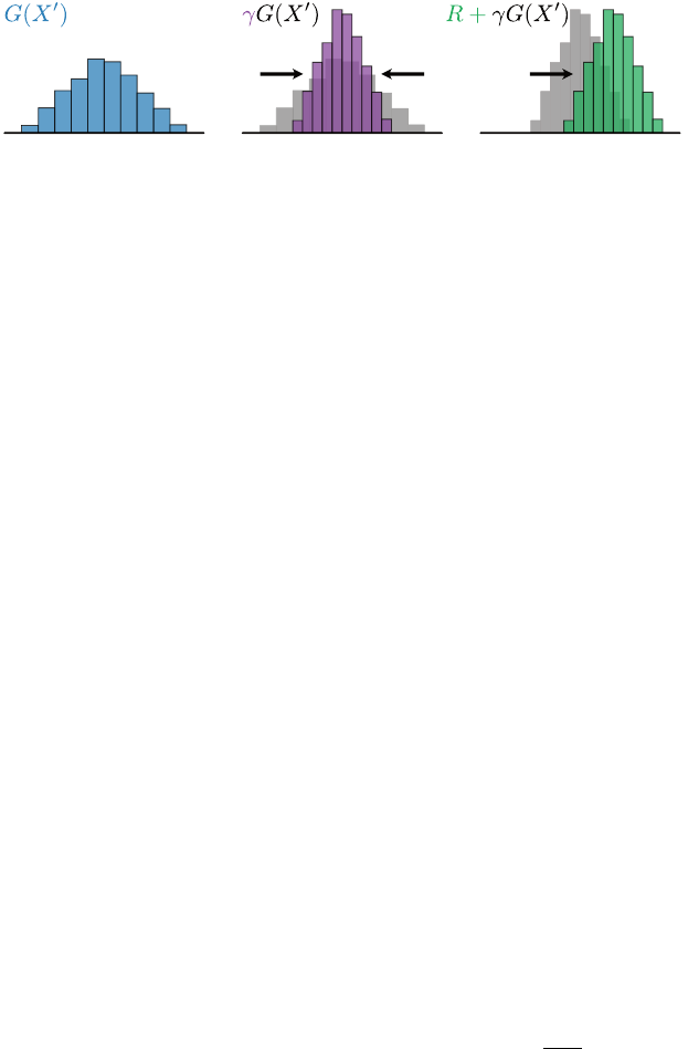
As in the expected-value setting, we construct a random-variable operator by
viewing the right-hand side of Equation 4.6 as a transformation of
G
π
. In this
case, we break down the transformation of
G
π
into three operations, each of
which produces a new random variable (Figure 4.1):
(a) G
π
(X
0
): the indexing of the collection of random variables G
π
by X
0
;
(b) γG
π
(
X
0
): the multiplication of the random variable
G
π
(
X
0
) with the scalar
γ;
(c) R + γG
π
(X
0
): the addition of two random variables (R and γG
π
(X
0
)).
More generally, we may apply these operations to any state-indexed collection
of random variables
G
=
G
(
x
) :
x ∈X
), taken to be independent of the random
transitions used to define the transformation. With some mathematical caveats
discussed below, let us introduce the random-variable Bellman operator
(T
π
G)(x)
D
= R + γG(X
0
), X = x . (4.7)
Equation 4.7 states that the application of the Bellman operator to
G
(evaluated
at
x
; the left-hand side) produces a random variable that is equal in distribution
to the random variable constructed on the right-hand side. Because this holds
for all
x
, we think of
T
π
as mapping
G
to a new collection of random variables
T
π
G.
The random-variable operator is appealing because it is concise and easily
understood. In many circumstances, this makes it the tool of choice for reasoning
about distributional reinforcement learning problems. One issue, however, is that
its definition above is mathematically incomplete. This is because it specifies
the probability distribution of (
T
π
G
)(
x
), but not its identity as a mapping from
some sample space to the real numbers. As discussed in Section 2.7, without
care we may produce random variables that exhibit undesirable behavior: for
example, because rewards at different points in time are improperly correlated.
More immediately, the theory of contraction mappings needs a clear definition
of the space on which an operator is defined – in the case of the random-variable
operator, this requires us to specify a space of random variables to operate
Draft version.
84 Chapter 4
(a) (b) (c)
Figure 4.1
The random-variable Bellman operator is composed of three operations:
(a)
indexing
into a collection of random variables,
(b)
multiplication by the discount factor, and
(c)
addition of two random variables. Here, we assume that
R
and
X
0
take on a single value
for clarity.
in. Properly defining such a space is possible but requires some technical
subtlety and measure-theoretic considerations; we refer the interested reader to
Section 4.9.
A more direct solution is to consider the distributional Bellman operator
as a mapping on the space of return-distribution functions. Starting with the
distributional Bellman equation
η
π
(x) = E
π
[
b
R,γ
#
η
π
(X
0
) |X = x] ,
we again view the right-hand side as the result of applying a series of
transformations, in this case to probability distributions.
Definition 4.8.
The distributional Bellman operator
T
π
:
P
(
R
)
X
→P
(
R
)
X
is
the mapping defined by
(T
π
η)(x) = E
π
[
b
R,γ
#
η(X
0
) |X = x] . (4.8)
4
Here, the operations on probability distributions are expressed (rather com-
pactly) by the expectation in Equation 4.8 and the use of the pushforward
distribution derived from the bootstrap function
b
; these are the operations of
mixing, scaling, and translation previously described in Section 2.8.
We can gain additional insight into how the operator transforms a return
function
η
by considering the situation in which the random reward
R
and the
return distributions
η
(
x
) admit respective probability densities
p
R
(
r | x, a
) and
p
x
(z). In this case, the probability density of (T
π
η)(x), denoted p
0
x
, is
p
0
x
(z) = γ
−1
X
a∈A
π(a | x)
Z
r∈R
p
R
(r | x, a)
X
x
0
∈X
P
X
(x
0
| x, a)p
x
0
z −r
γ
dr . (4.9)
Expressed in terms of probability densities, the indexing of a collection of
random variables becomes a mixture of densities, while their addition becomes a
Draft version.

Operators and Metrics 85
convolution; this is in fact what is depicted in Figure 4.1. In terms of cumulative
distribution functions, we have
F
(T
π
η)(x)
(z) = E
π
h
F
η(X
0
)
z −R
γ
| X = x
i
.
However, we prefer the operator that deals directly with probability distributions
(Equation 4.8) as it can be used to concisely express more complex operations on
distributions. One such operation is the projection of a probability distribution
onto a finitely parameterized set, which we will use in Chapter 5 to construct
algorithms for approximating η
π
.
Using Definition 4.8, we can formally express the fact that the return-
distribution function η
π
is the only solution to the equation
η = T
π
η .
The proof is relatively technical and will be given in Section 4.8.
Proposition 4.9. The return-distribution function η
π
satisfies
η
π
= T
π
η
π
and is the unique fixed point of the distributional Bellman operator
T
π
.
4
When working with the distributional Bellman operator, one should be mind-
ful that the random reward
R
and next state
X
0
are generally not independent,
because they both depend on the chosen action
A
(we briefly mentioned this
concern in Section 2.8). In Equation 4.9, this is explicitly handled by the outer
sum over actions. Analogously, we can make explicit the dependency on
A
by
introducing a second expectation in Equation 4.8:
(T
π
η)(x) = E
π
E
π
[(b
R,γ
)
#
η(X
0
) |X = x, A] |X = x
.
By conditioning the inner expectation on the action
A
, we make the random
variables
R
and
γG
(
X
0
) conditionally independent in the inner expectation. We
will make use of this technique in proving Theorem 4.25, the main theoretical
result of this chapter.
In some circumstances, it is useful to translate between operations on proba-
bility distributions and those on random variables. We do this by means of a
representative set of random variables called an instantiation.
Definition 4.10.
Given a probability distribution
ν ∈P
(
R
), we say that a ran-
dom variable
Z
is an instantiation of
ν
if its distribution is
ν
, written
Z ∼ν
.
Similarly, we say that a collection of random variables
G
= (
G
(
x
) :
x ∈X
) is an
instantiation of a return-distribution function
η ∈P
(
R
)
X
if for every
x ∈X
, we
have G(x) ∼η(x). 4
Draft version.

86 Chapter 4
Given a return-distribution function
η ∈P
(
R
)
X
, the new return-distribution
function
T
π
η
can be obtained by constructing an instantiation
G
of
η
, perform-
ing the transformation on the collection of random variables
G
as described
at the beginning of this section, and then extracting the distributions of the
resulting random variables. This is made formal as follows.
Proposition 4.11.
Let
η ∈P
(
R
)
X
, and let
G
= (
G
(
x
) :
x ∈X
) be an instan-
tiation of
η
. For each
x ∈X
, let (
X
=
x, A, R, X
0
) be a sample transition
independent of G. Then R + γG(X
0
) has the distribution (T
π
η)(x):
D
π
(R + γG(X
0
) | X = x) = (T
π
η)(x) . 4
Proof.
The result follows immediately from the definition of the distributional
Bellman operator. For clarity, we step through the argument again, mirroring
the transformations set out at the beginning of the section. First, the indexing
transformation gives
D
π
(G(X
0
) | X = x) =
X
x
0
∈X
P
π
(X
0
= x
0
| X = x)η(x
0
)
= E
π
[η(X
0
) | X = x] .
Next, scaling by γ yields
D
π
(γG(X
0
) | X = x) = E
π
[(b
0,γ
)
#
η(X
0
) | X = x] ,
and finally adding the immediate reward R gives the result
D
π
(R + γG(X
0
) | X = x) = E
π
[(b
R,γ
)
#
η(X
0
) | X = x] .
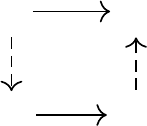
Proposition 4.11 is an instance of a recurring principle in distributional rein-
forcement learning that “different routes lead to the same answer.” Throughout
this book, we will illustrate this point as it arises with a commutative diagram;
the particular case under consideration is depicted in Figure 4.2.
4.4 Wasserstein Distances for Return Functions
Many desirable properties of reinforcement learning algorithms (for example,
the fact that they produce a good approximation of the value function) are
due to the contractive nature of the Bellman operator
T
π
. In this section, we
will establish that the distributional Bellman operator
T
π
, too, is a contraction
mapping – analogous to the value-based operator, the application of
T
π
brings
return functions closer together.
One difference between expected-value and distributional reinforcement
learning is that the space of return-distribution functions
P
(
R
)
X
is substantially
Draft version.
Operators and Metrics 87
η η
0
G G
0
T
π
T
π
Figure 4.2
A commutative diagram illustrating two perspectives on the application of the distri-
butional Bellman operator. The top horizontal line represents the direct application to
the return-distribution function
η
, yielding
η
0
. The alternative path first instantiates the
return-distribution function
η
as a collection of random variables
G
= (
G
(
x
) : (
x
)
∈X
),
transforms
G
to obtain another collection of random variables
G
0
, and then extracts the
distributions of these random variables to obtain η
0
.
different from the space of value functions. To measure distances between value
functions, we can simply treat them as finite-dimensional vectors, taking the
absolute difference of value estimates at individual states. By contrast, it is
somewhat less intuitive to see what “close” means when comparing probability
distributions. Throughout this chapter, we will consider a number of probability
metrics that measure distances between distributions, each presenting differ-
ent mathematical and computational properties. We begin with the family of
Wasserstein distances.
Definition 4.12.
Let
ν ∈P
(
R
) be a probability distribution with cumulative
distribution function
F
ν
. Let
Z
be an instantiation of
ν
(in particular,
F
Z
=
F
ν
).
The generalized inverse F
−1
ν
is given by
F
−1
ν
(τ) = inf
z∈R
{z : F
ν
(z) ≥τ}.
We additionally write F
−1
Z
= F
−1
ν
. 4
Definition 4.13.
Let
p ∈
[1
, ∞
). The
p
-Wasserstein distance is a function
w
p
:
P(R) ×P(R) →[0, ∞] given by
w
p
(ν, ν
0
) =
Z
1
0
F
−1
ν
(τ) −F
−1
ν
0
(τ)
p
dτ
!
1/p
.
The ∞-Wasserstein distance w
∞
: P(R) ×P(R) →[0, ∞] is
w
∞
(ν, ν
0
) = sup
τ∈(0,1)
F
−1
ν
(τ) − F
−1
ν
0
(τ)
. 4
Graphically, the Wasserstein distances between two probability distributions
measure the area between their cumulative distribution functions, with val-
ues along the abscissa taken to the
p
th power; see Figure 4.3. When
p
=
∞
,
Draft version.

88 Chapter 4
this becomes the largest horizontal difference between the inverse cumulative
distribution functions. The
p
-Wasserstein distances satisfy the definition of a
metric, except that they may not be finite for arbitrary pairs of distributions
in
P
(
R
); see Exercise 4.6. Properly speaking, they are said to be extended
metrics, since they may take values on the real line extended to include infinity.
Most probability metrics that we will consider are extended metrics rather than
metrics in the sense of Definition 4.2. We measure distances between return-
distribution functions in terms of the largest Wasserstein distance between
probability distributions at individual states.
Definition 4.14.
Let
p ∈
[1
, ∞
]. The supremum
p
-Wasserstein distance
w
p
between two return-distribution functions η, η
0
∈P(R)
X
is defined by
27
w
p
(η, η
0
) = sup
x∈X
w
p
(η(x), η
0
(x)) . 4
The supremum
p
-Wasserstein distances fulfill all requirements of an extended
metric on the space of return-distribution functions
P
(
R
)
X
; see Exercise 4.7.
Based on these distances, we give our first contractivity result regarding the
distributional Bellman operator; its proof is given at the end of the section.
Proposition 4.15.
The distributional Bellman operator is a contraction
mapping on
P
(
R
)
X
in the supremum
p
-Wasserstein distance, for all
p ∈
[1, ∞]. More precisely,
w
p
(T
π
η, T
π
η
0
) ≤γw
p
(η, η
0
) ,
for all η, η
0
∈P (R)
X
. 4
Proposition 4.15 is significant in that it establishes a close parallel between
the expected-value and distributional operators. Following the line of reasoning
given in Section 4.2, it provides the mathematical justification for the develop-
ment and analysis of computational approaches for finding the return function
η
π
. More immediately, it also enables us to characterize the convergence of the
sequence
η
k+1
= T
π
η
k
(4.10)
to the return function η
π
.
27.
Because we assume that there are finitely many states, we can equivalently write
max
in the
definition of supremum distance. However, we prefer the more generally applicable sup.
Draft version.
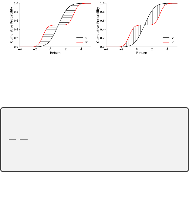
Operators and Metrics 89
Figure 4.3
Left
: Illustration of the
p
-Wasserstein distance between a normal distribution
ν
=
N
(1
,
1)
and a mixture of two normal distributions
ν
0
=
1
2
N
(
−
1
,
0
.
5) +
1
2
N
(3
,
0
.
5).
Right
: Illus-
tration of the
p
metric for the same distributions (see Section 4.5). In both cases, the
shading indicates the axis along which the differences are taken to the pth exponent.
Proposition 4.16.
Suppose that for each (
x, a
)
∈X×A
, the reward distri-
bution
P
R
(
· | x, a
) is supported on the interval [
R
min
, R
max
]. Then for any
initial return function
η
0
whose distributions are bounded on the interval
h
R
min
1−γ
,
R
max
1−γ
i
, the sequence
η
k+1
= T
π
η
k
converges to
η
π
in the supremum
p
-Wasserstein distance (for all
p ∈
[1
, ∞
]).
4
The restriction to bounded rewards in Proposition 4.16 is necessary to make
use of the tools developed in Section 4.2, at least without further qualification.
This is because Proposition 4.7 requires all distances to be finite, which is not
guaranteed under our definition of a probability metric. If, for example, the
initial condition η
0
is such that
w
p
(η
0
, η
π
) = ∞,
then Proposition 4.15 is not of much use. A less restrictive but more technically
elaborate set of assumptions will be presented later in the chapter. For now, we
provide the proof of the two preceding results. First, we obtain a reasonably
simple proof of Proposition 4.15 by considering an alternative formulation of
the p-Wasserstein distances in terms of couplings.
Definition 4.17.
Let
ν, ν
0
∈P
(
R
) be two probability distributions. A coupling
between
ν
and
ν
0
is a joint distribution
υ ∈P
(
R
2
) such that if (
Z, Z
0
) is an
instantiation of
υ
, then also
Z
has distribution
ν
and
Z
0
has distribution
ν
0
. We
write Γ(ν, ν
0
) ⊆P(R
2
) for the set of all couplings of ν and ν
0
. 4
Draft version.

90 Chapter 4
Proposition 4.18
(see Villani (2008) for a proof)
.
Let
p ∈
[1
, ∞
).
Expressed in terms of an optimal coupling, the
p
-Wasserstein distance
between two distributions ν, ν
0
∈P (R) is
w
p
(ν, ν
0
) = min
υ∈Γ(ν,ν
0
)
E
(Z,Z
0
)∼υ
[|Z −Z
0
|
p
]
1/p
.
The ∞-Wasserstein distance between ν and ν
0
can be written as
w
∞
(ν, ν
0
) = min
υ∈Γ(ν,ν
0
)
inf
n
z ∈R :
P
(Z,Z
0
)∼υ
(|Z −Z
0
|> z) = 0
o
. 4
Informally, the optimal coupling finds an arrangement of the two probability
distributions that maximizes “agreement”: it produces outcomes that are as close
as possible. In Proposition 4.18, the optimal coupling takes on a very simple
form given by inverse cumulative distribution functions. For
ν, ν
0
∈P
(
R
), an
optimal coupling is the probability distribution of the random variable
F
−1
ν
(τ), F
−1
ν
0
(τ)
, τ ∼U
[0, 1]
. (4.11)
This can be understood by noting how the 1-Wasserstein distance between
ν
and
ν
0
is obtained by measuring the horizontal distance between the two cumulative
distribution functions, at each level τ ∈[0, 1] (Figure 4.3).
Proof of Proposition 4.15.
Let
p ∈
[1
, ∞
) be fixed. For each
x ∈X
, consider the
optimal coupling between
η
(
x
) and
η
0
(
x
) and instantiate it as the pair of ran-
dom variables
G
(
x
)
, G
0
(
x
)
. Next, denote by (
x, A, R, X
0
) the random transition
beginning in
x ∈X
, constructed to be independent from
G
(
y
) and
G
0
(
y
), for all
y ∈X. With these variables, write
˜
G(x) = R + γG(X
0
) ,
˜
G
0
(x) = R + γG
0
(X
0
) .
By Proposition 4.11,
˜
G(x) has distribution (T
π
η)(x) and
˜
G
0
(x) has distribution
(
T
π
η
0
)(
x
). The pair
˜
G
(
x
)
,
˜
G
0
(
x
)
therefore forms a valid coupling of these
distributions. Now
w
p
p
(T
π
η)(x), (T
π
η
0
)(x)
(a)
≤ E
π
h
R + γG(X
0
)
−
R + γG
0
(X
0
)
p
| X = x
i
(b)
= γ
p
E
h
G(X
0
) −G
0
(X
0
)
p
| X = x
i
(c)
≤ γ
p
X
x
0
∈X
P
π
(X
0
= x
0
| X = x) E
h
G(x
0
) −G
0
(x
0
)
p
i
(d)
≤ γ
p
sup
x
0
∈X
E
h
G(x
0
) −G
0
(x
0
)
p
i
(e)
= γ
p
w
p
p
(η, η
0
) .
Draft version.

Operators and Metrics 91
Taking a supremum over
x ∈X
on the left-hand side and the
p
th root of both
sides yields the result. Here, (a) follows since the Wasserstein distance is
defined as a minimum over couplings, (b) follows from algebraic manipulation
of the expectation, (c) follows from independence of the sample transition
(
X
=
x, A, R, X
0
) and the random variables (
G
(
x
)
, G
0
(
x
) :
x ∈X
), (d) because the
maximum of nonnegative quantities is at least as great as their weighted average,
and (e) follows since (
G
(
x
0
)
, G
0
(
x
0
)) was defined as an optimal coupling of
η
(
x
0
)
and η
0
(x
0
). The proof for p = ∞ is similar (see Exercise 4.8).
Proof of Proposition 4.16.
Let us denote by
P
B
(
R
) the space of distributions
bounded on [V
min
, V
max
], where as usual
V
min
=
R
min
1 −γ
, V
max
=
R
max
1 −γ
.
We will show that under the assumption of rewards bounded on [R
min
, R
max
],
(a) the return function η
π
is in P
B
(R), and
(b) the distributional Bellman operator maps P
B
(R) to itself.
Consequently, we can invoke Proposition 4.7 with
O
=
T
π
and
M
=
P
B
(
R
)
to conclude that for any initial
η
0
∈P
B
(
R
)
X
, the sequence of iterates (
η
k
)
k≥0
converges to η
π
with respect to d = w
p
, for any p ∈[1, ∞].
To prove (a), note that for any state x ∈X,
G
π
(x) =
∞
X
t=0
γ
t
R
t
, X
0
= x ,
and since
R
t
∈
[
R
min
, R
max
] for all
t
, then also
G
π
(
x
)
∈
[
V
min
, V
max
]. For (b), let
η ∈P
B
(
R
)
X
and denote by
G
an instantiation of this return-distribution function.
For any x ∈X,
P
π
R + γG(X
0
) ≤V
max
| X = x
= P
π
γG(X
0
) ≤V
max
−R | X = x
≥P
π
γG(X
0
) ≤V
max
−R
max
| X = x
= P
π
G(X
0
) ≤V
max
| X = x
= 1.
By the same reasoning,
P
π
R + γG(X
0
) ≥V
min
| X = x
= 1.
Since
R
+
γG
(
X
0
)
, X
=
x
is an instantiation of (
T
π
η
)(
x
) for each
x
, we conclude
that if η ∈P
B
(R)
X
, then also T
π
η ∈P
B
(R)
X
.
Draft version.

92 Chapter 4
4.5 `
p
Probability Metrics and the Cramér Distance
The previous section established that the distributional Bellman operator is well
behaved with respect to the family of Wasserstein distances. However, these
are but a few among many standard probability metrics. We will see in Chapter
5 that theoretical analysis sometimes requires us to study the behavior of the
distributional operator with respect to other metrics. In addition, many practical
algorithms directly optimize a metric (typically expressed as a loss function) as
part of their operation (see Chapter 10). The Cramér distance, a member of the
broader family of
p
metrics, is of particular interest to us.
Definition 4.19.
Let
p ∈
[1
, ∞
). The distance
p
:
P
(
R
)
×P
(
R
)
→
[0
, ∞
] is a
probability metric defined by
p
(ν, ν
0
) =
Z
R
|F
ν
(z) −F
ν
0
(z)|
p
dz
!
1/p
. (4.12)
For
p
= 2, this is the Cramér distance.
28
The
∞
or Kolmogorov–Smirnov
distance is given by
∞
(ν, ν
0
) = sup
z∈R
F
ν
(z) −F
ν
0
(z)
.
The respective supremum
p
distances are given by (η, η
0
∈P(R)
X
)
p
(η, η
0
) = sup
x∈X
p
η(x), η(x
0
)
.
These are extended metrics on P(R)
X
. 4
Where the
p
-Wasserstein distances measure differences in outcomes, the
p
distances measure differences in the probabilities associated with these
outcomes. This is because the exponent
p
is applied to cumulative probabilities
(this is illustrated in Figure 4.3). The distributional Bellman operator is also a
contraction mapping under the
p
distances for
p ∈
[1
, ∞
), albeit with a larger
contraction modulus.
29
28.
Historically, the Cramér distance has been defined as the square of
2
. In our context, it seems
unambiguous to use the word for
2
itself.
29.
For
p
= 1, the distributional Bellman operator has contraction modulus
γ
; this is sensible given
that
1
= w
1
.
Draft version.

Operators and Metrics 93
Proposition 4.20.
For
p ∈
[1
, ∞
), the distributional Bellman operator
T
π
is a contraction mapping on
P
(
R
)
X
with respect to
p
, with contraction
modulus γ
1
/p
. That is,
p
(T
π
η, T
π
η
0
) ≤γ
1
/p
p
(η, η
0
)
for all η, η
0
∈P (R)
X
. 4
The proof of Proposition 4.20 will follow as a corollary of a more general
result given in Section 4.6. One way to relate it to our earlier result is to consider
the behavior of the sequence defined by
η
k+1
= T
π
η
k
. (4.13)
As measured in the
p
-Wasserstein distance, the sequence (
η
k
)
k≥0
approaches
η
π
at a rate of
γ
; but if we instead measure distances using the
p
metric, this
rate is slower – only
γ
1
/p
. Measured in terms of
∞
(the Kolmogorov–Smirnov
distance), the sequence of iterates may in fact not seem to approach
η
π
at all.
To see this, it suffices to consider a single-state process with zero reward (that
is,
P
X
(
X
0
=
x | X
=
x
) = 1 and
R
= 0) and a discount factor
γ
= 0
.
9. In this case,
η
π
(x) = δ
0
. For the initial condition η
0
(x) = δ
1
, we obtain
η
1
(x) = (T
π
η
0
)(x) = δ
γ
.
Now, the (supremum)
∞
distance between
η
π
and
η
0
is 1, because for any
z ∈(0, 1),
F
η
0
(x)
(z) = 0 F
η
π
(x)
(z) = 1.
However, the
∞
distance between
η
π
and
η
1
is also 1, by the same argument
(but now restricted to z ∈(0, γ)). Hence, there is no β ∈[0, 1) for which
∞
(η
1
, η
π
) < β
∞
(η
0
, η
π
).
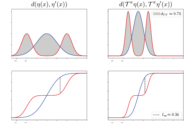
Exercise 4.16 asks you to prove a similar result for a probability metric called
the total variation distance (see also Figure 4.4).
The more general point is that different probability metrics are sensitive to
different characteristics of probability distributions, and to varying degrees.
At one extreme, the
∞
-Wasserstein distance is effectively insensitive to the
probability associated with different outcomes, while at the other extreme,
the Kolmogorov–Smirnov distance is insensitive to the scale of the difference
between outcomes. In Section 4.6, we will show that a metric’s sensitivity to
differences in outcomes determines the contraction modulus of the distributional
Bellman operator under that metric; informally speaking, this explains the “nice”
behavior of the distributional Bellman operator under the Wasserstein distances.
Draft version.
94 Chapter 4
0.2
0.4
0.6
0.8
0.2
0.4
0.6
0.8
Probability Density
2 1 0 1 2 3 4 5
Return
0.0
Probability Density
2 1 0 1 2 3 4 5
Return
0.0
2 1 0 1 2 3 4 5
Return
0.0
0.2
0.4
0.6
0.8
1.0
Cumulative Probability
2 1 0 1 2 3 4 5
Return
0.0
0.2
0.4
0.6
0.8
1.0
Cumulative Probability
(a) (b)
(c) (d)
Figure 4.4
The distributional Bellman operator is not a contraction mapping in either the supremum
form of
(a, b)
total variation distance (
d
TV
, shaded in the top panels; see Exercise
4.16 for a definition) or
(c, d)
Kolmogorov–Smirnov distance
∞
(vertical distance in
the bottom panels). The left panels show the density
(a)
and cumulative distribution
function
(c)
of two distributions
η
(
x
) (blue) and
η
0
(
x
) (red). The right panels show the
same after applying the distributional Bellman operator
(b, d)
, specifically considering
the transformation induced by the discount factor
γ
. The lack of contractivity can be
explained by the fact that neither
d
TV
nor
∞
is a homogeneous probability metric
(Section 4.6).
Before moving on, let us summarize the results established thus far. By
combining the theory of contraction mappings with suitable probability metrics,
we were able to characterize the behavior of the iterates
η
k+1
= T
π
η
k
. (4.14)
In the following chapters, we will use this as the basis for the design of
implementable algorithms that approximate the return distribution
η
π
and will
appeal to contraction mapping theory to provide theoretical guarantees for these
algorithms. In particular, in Chapter 6, we will analyze the categorical temporal-
difference learning under the lens of the Cramér distance. While the results
presented until now suffice for most practical purposes, the following sections
Draft version.

Operators and Metrics 95
deal with some of the more technical considerations that arise from study-
ing Equation 4.14 under general conditions, particularly the issue of infinite
distances between distributions.
4.6 Sufficient Conditions for Contractivity
In the remainder of this chapter, we characterize in greater generality the
behavior of the sequence of return function estimates described by Equation
4.14, viewed under the lens of different probability metrics. We begin with a
formal definition of what it means for a function d to be a probability metric.
Definition 4.21.
A probability metric is an extended metric on the space of
probability distributions, written
d : P(R) ×P(R) →[0, ∞] .
Its supremum extension is the function d : P(R)
X
×P(R)
X
→R defined as
d(η, η
0
) = sup
x∈X
d(η(x), η
0
(x)) .
We refer to
d
as a return-function metric; it is an extended metric on
P
(
R
)
X
.
4
Our analysis is based on three properties that a probability metric should
possess in order to guarantee contractivity. These three properties relate closely
to the three fundamental operations that make up the distributional Bellman
operator: scaling, convolution, and mixture of distributions (equivalently: scal-
ing, addition, and indexing of random variables). In this analysis, we will find
that some properties are more easily stated in terms of random variables, oth-
ers in terms of probability distributions. Accordingly, given two probability
distributions ν, ν
0
with instantiations Z, Z
0
, let us overload notation and write
d(Z, Z
0
) = d(ν, ν
0
).
Definition 4.22.
Let
c >
0. The probability metric
d
is
c
-homogeneous if for any
scalar
γ ∈
[0
,
1) and any two distributions
ν, ν
0
∈P
(
R
) with associated random
variables Z, Z
0
, we have
d(γZ, γZ
0
) = γ
c
d(Z, Z
0
) .
In terms of probability distributions, this is equivalently given by the condition
d((b
0,γ
)
#
ν, (b
0,γ
)
#
ν
0
) = γ
c
d(ν, ν
0
) .
If no such c exists, we say that d is not homogeneous. 4
Definition 4.23.
The probability metric
d
is regular if for any two distributions
ν, ν
0
∈P
(
R
) with associated random variables
Z, Z
0
, and an independent random
Draft version.

96 Chapter 4
variable W, we have
d(W + Z, W + Z
0
) ≤d(Z, Z
0
) . (4.15)
In terms of distributions, this is
d
E
W
[(b
W,1
)
#
ν], E
W
[(b
W,1
)
#
ν
0
]
≤d(ν, ν
0
) . 4
Definition 4.24.
Given
p ∈
[1
, ∞
), the probability metric
d
is
p
-convex
30
if for
any α ∈(0, 1) and distributions ν
1
, ν
2
, ν
0
1
, ν
0
2
∈P(R), we have
d
p
αν
1
+ (1 −α)ν
2
, αν
0
1
+ (1 −α)ν
0
2
≤αd
p
(ν
1
, ν
0
1
) + (1 −α)d
p
(ν
2
, ν
0
2
) . 4
Although this
p
-convexity property is given for a mixture of two distributions,
it implies an analogous property for mixtures of finitely many distributions.
Theorem 4.25.
Consider a probability metric
d
. Suppose that
d
is regular,
c
-homogeneous for some
c >
0, and that there exists
p ∈
[1
, ∞
) such that
d
is
p
-convex. Then for all return-distribution functions
η, η
0
∈P
(
R
)
X
, we
have
d(T
π
η, T
π
η
0
) ≤γ
c
d(η, η
0
) . 4
Proof.
Fix a state
x ∈X
and action
a ∈A
. For this state, consider the sample
transition (
X
=
x, A
=
a, R, X
0
) (Equation 2.12), and recall that
R
and
X
0
are
independent given X and A, since
R ∼P
R
( · | X, A) X
0
∼P
X
( · | X, A) .
Let
G
and
G
0
be instantiations of
η
and
η
0
, respectively.
31
We introduce a state-
action variant of the distributional Bellman operator,
T
:
P
(
R
)
X
→P
(
R
)
X×A
,
given by
(Tη)(x, a) = E[(b
R,γ
)
#
η(X
0
) |X = x, A = a].
Note that this operator is defined independently of the policy
π
, since the action
a
is specified as an argument. We then calculate directly, indicating where each
hypothesis of the result is used:
d
p
((Tη)(x, a), (Tη
0
)(x, a)) = d
p
R + γG(X
0
), R + γG
0
(X
0
)
(a)
≤ d
p
γG(X
0
), γG
0
(X
0
)
(b)
= γ
pc
d
p
G(X
0
), G
0
(X
0
)
30.
This matches the usual definition of convexity (for
d
p
) if one treats the pair (
ν
1
, ν
2
) as a single
argument from P(R) ×P(R).
31. Note: the proof does not assume the independence of G(x) and G(y), x , y. See Exercise 4.12.
Draft version.

Operators and Metrics 97
(c)
≤ γ
pc
X
x
0
∈X
P
π
(X
0
= x
0
| X = x, A = a)d
p
G(x
0
), G
0
(x
0
)
≤γ
pc
sup
x
0
∈X
d
p
G(x
0
), G
0
(x
0
)
= γ
pc
d
p
(η, η
0
) .
Here, (a) follows from regularity of
d
, (b) follows from the
c
-homogeneous
property of
d
, and (c) follows from
p
-convexity, where the mixture is over the
values taken by the random variable X
0
. We also note that
(T
π
η)(x) =
X
a∈A
π(a | x)(Tη)(x, a),
and hence by p-convexity of d, we have
d
p
(T
π
η)(x), (T
π
η
0
)(x)
≤
X
a∈A
π(a | x)d
p
(T
π
η)(x, a), (T
π
η
0
)(x, a)
≤γ
pc
d
p
(η, η
0
) .
Taking the supremum over
x ∈X
on the left-hand side and taking
p
th roots then
yields the result.
Theorem 4.25 illustrates how the contractivity of the distributional Bellman
operator in the probability metric
d
(specifically, in its supremum extension)
follows from natural properties of
d
. We see that the contraction modulus is
closely tied to the homogeneity of
d
, which informally characterizes the extent
to which scaling random variables by a factor
γ
brings them “closer together.”
The theorem provides an alternative to our earlier result regarding Wasserstein
distances and enables us to establish the contractivity under the
p
distances but
also under other probability metrics. Exercise 4.19 explores contractivity under
the so-called maximum mean discrepancy (MMD) family of distances.
Proof of Proposition 4.20 (contractivity in
p
distances).
We will apply Theo-
rem 4.25 to the probability metric
p
, for
p ∈
[1
, ∞
). It is therefore sufficient to
demonstrate that
p
is
1
/p-homogeneous, regular, and p-convex.
1/p-homogeneity.
Let
ν, ν
0
∈P
(
R
) with associated random variables
Z, Z
0
.
We make use of the fact that for γ ∈[0, 1),
F
γZ
(z) = F
Z
z
γ
.
Writing
p
p
for the pth power of
p
, we have
p
p
(γZ, γZ
0
) =
Z
R
F
γZ
(z) −F
γZ
0
(z)
p
dz
Draft version.

98 Chapter 4
=
Z
R
F
Z
(
z
γ
) −F
Z
0
(
z
γ
)
p
dz
(a)
=
Z
R
γ
F
Z
(z) −F
Z
0
(z)
p
dz
= γ
p
p
(Z, Z
0
) , (4.16)
where (a) follows from a change of variables
z/γ 7→z
in the integral. Therefore,
we deduce that
p
(γZ, γZ
0
) = γ
1/p
p
(Z, Z
0
).
Regularity.
Let
ν, ν
0
∈P
(
R
), with
Z, Z
0
independent instantiations of
ν
and
ν
0
, respectively, and let W be a random variable independent of Z, Z
0
. Then,
p
p
(W + Z, W + Z
0
) =
Z
R
|F
W+Z
(z) −F
W+Z
0
(z)|
p
dz
=
Z
R
|E
W
[F
Z
(z −W)] −E
W
[F
Z
0
(z −W)]|
p
dz
(a)
≤
Z
R
E
W
[|F
Z
(z −W) −F
Z
0
(z −W)|
p
]dz
(b)
= E
W
Z
R
|F
Z
(z −W) −F
Z
0
(z −W)|
p
]dz
=
p
p
(Z, Z
0
) ,
where (a) follows from Jensen’s inequality, and (b) follows by swapping the
integral and expectation (more formally justified by Tonelli’s theorem).
p-convexity. Let α ∈(0, 1), and ν
1
, ν
0
1
, ν
2
, ν
0
2
∈P (R). Note that
F
αν
1
+(1−α)ν
2
(z) = αF
ν
1
(z) + (1 −α)F
ν
2
(z) ,
and similarly for the primed distributions
ν
0
1
, ν
0
2
. By convexity of the function
z 7→|z|
p
on the real numbers and Jensen’s inequality,
|F
αν
1
+(1−α)ν
2
(z) −F
αν
0
1
+(1−α)ν
0
2
(z)|
p
≤α|F
ν
1
(z) −F
ν
0
1
(z)|
p
+ (1 −α)|F
ν
2
(z) −F
ν
0
2
(z)|
p
,
for all z ∈R. Hence,
p
p
(αν
1
+ (1 −α)ν
2
, αν
0
1
+ (1 −α)ν
0
2
) ≤ α
p
p
(ν
1
, ν
0
1
) + (1 −α)
p
p
(ν
2
, ν
0
2
),
and
p
is p-convex.
4.7 A Matter of Domain
Suppose that we have demonstrated, by means of Theorem 4.25, that the distri-
butional Bellman operator is a contraction mapping in the supremum extension
Draft version.
Operators and Metrics 99
of some probability metric d. Is this sufficient to guarantee that the sequence
η
k+1
= T
π
η
k
converges to the return function
η
π
, by means of Proposition 4.7? In general,
no, because
d
may assign infinite distances to certain pairs of distributions.
To invoke Proposition 4.7, we identify a subset of probability distributions
P
d
(
R
) that are all within finite
d
-distance of each other and then ensure that
the distributional Bellman operator is well behaved on this subset. Specifically,
we identify a set of conditions under which
(a) the distributional Bellman operator T
π
maps P
d
(R)
X
to itself, and
(b) the return function η
π
(the fixed point of T
π
) lies in P
d
(R)
X
.
For most common probability metrics and natural problem settings, these
requirements are easily verified. In Proposition 4.16, for example, we demon-
strated that under the assumption that the reward distributions are bounded,
then Proposition 4.7 can be applied with the Wasserstein distances. The aim of
this section is to extend the analysis to a broader set of probability metrics but
also to a greater number of problem settings, including those where the reward
distributions are not bounded.
Definition 4.26.
Let
d
be a probability metric. Its finite domain
P
d
(
R
)
⊆P
(
R
)
is the set of probability distributions with finite first moment and finite
d
-
distance to the distribution that puts all of its mass on zero:
P
d
(R) =
ν ∈P(R) : d(ν, δ
0
) < ∞, E
Z∼ν
[|Z|] < ∞
. (4.17)
4
By the triangle inequality, for any two distributions
ν, ν
0
∈P
d
(
R
), we are
guaranteed
d
(
ν, ν
0
)
< ∞
. Although the choice of
δ
0
as the reference point is some-
what arbitrary, it is sensible given that many reinforcement learning problems
include the possibility of receiving no reward at all (e.g.,
G
π
(
x
) = 0). The finite
first-moment assumption is made in light of Assumption 2.5, which guarantees
that return distributions have well-defined expectations.
Draft version.

100 Chapter 4
Proposition 4.27.
Let
d
be a probability metric satisfying the conditions
of Theorem 4.25, with finite domain
P
d
(
R
). Let
T
π
be the distribu-
tional Bellman operator corresponding to a given Markov decision process
(X, A, ξ
0
, P
X
, P
R
). Suppose that
(a) η
π
∈P
d
(R), and
(b) P
d
(
R
) is closed under
T
π
: for any
η ∈P
d
(
R
)
X
, we have that
T
π
η ∈
P
d
(R)
X
.
Then for any initial condition
η
0
∈P
d
(
R
), the sequence of iterates defined
by
η
k+1
= T
π
η
k
converges to η
π
with respect to d. 4
Proposition 4.27 is a specialization of Proposition 4.7 to the distributional
setting and generalizes our earlier result regarding bounded reward distributions.
Effectively, it allows us to prove the convergence of the sequence (
η
k
)
k≥0
for a
family of Markov decision processes satisfying the two conditions above. The
condition
η
π
∈P
d
(
R
), while seemingly benign, does not automatically hold;
Exercise 4.20 illustrates the issue using a modified p-Wasserstein distance.
Example 4.28
(
p
metrics)
.
For a given
p ∈
[1
, ∞
), the finite domain of the
probability metric
p
is
P
p
(R) = {ν ∈P(R) : E
Z∼ν
[|Z|] < ∞},
the set of distributions with finite first moment. This follows because
p
p
(ν, δ
0
) =
Z
0
−∞
F
ν
(z)
p
dz +
Z
∞
0
(1 −F
ν
(z))
p
dz
≤
Z
0
−∞
F
ν
(z)dz +
Z
∞
0
(1 −F
ν
(z))dz
(a)
= E[max(0, −Z)] + E[max(0, Z)]
= E[|Z|] ,
where (
a
) follows from expressing
F
ν
(
z
) and 1
−F
ν
(
z
) as integrals and using
Tonelli’s theorem:
Z
∞
0
(1 −F
ν
(z))dz =
Z
∞
0
E
Z∼ν
[ {Z > z}]dz
= E
Z∼ν
h
Z
∞
0
{Z > z}dz
i
Draft version.

Operators and Metrics 101
= E
Z∼ν
[max(0, Z)] ,
and similarly for the integral from −∞ to 0.
The conditions of Proposition 4.27 are guaranteed by Assumption 2.5
(rewards have finite first moments). From Chapter 2, we know that under
this assumption, the random return has finite expected value and hence
η
π
(x) ∈P
p
(R), for all x ∈X.
Similarly, we can show from elementary operations that if R and G(x) satisfy
E
π
|R|
X = x] < ∞, E[|G(x)|
< ∞, for all x ∈X,
then also
E
π
|R + γG(X
0
)|
X = x
< ∞, for all x ∈X.
Following Proposition 4.27, provided that
η
0
∈P
p
(
R
)
X
, then the sequence
(η
k
)
k≥0
converges to η
π
with respect to
p
. 4
When
d
is the
p
-Wasserstein distance (
p ∈
[1
, ∞
]), the finite domain takes on
a particularly useful form that we denote by P
p
(R):
P
p
(R) =
ν ∈P(R) : E
Z∼ν
[|Z|
p
] < ∞
, p ∈[0, ∞) ,
P
∞
(R) =
ν ∈P(R) : ∃C > 0 s.t. ν([−C, C]) = 1
.
For
p < ∞
, this is the set of distributions with bounded
p
th moments; for
p
=
∞
,
the set of distributions with bounded support. In particular, observe that the
finite domains of
1
and w
1
coincide: P
p
(R) = P
1
(R).
As with the
p
distances, we can satisfy the conditions of Proposition 4.27
for
d
=
w
p
by introducing an assumption on the reward distributions. In this
case, we simply require that these be in
P
p
(
R
). As this assumption will recur
throughout the book, we state it here in full; Exercise 4.11 goes through the
steps of the corresponding result.
Assumption 4.29(p).
For each state-action pair (
x, a
)
∈X×A
, the reward
distribution P
R
( · | x, a) is in P
p
(R). 4
Proposition 4.30.
Let
p ∈
[1
, ∞
]. Under Assumption 4.29(
p
), the return
function
η
π
has finite
p
th moments (
p
=
∞
: is bounded). In addition, for
any initial return function η
0
∈P
p
(R), the sequence defined by
η
k+1
= T
π
η
k
converges to η
π
with respect to the supremum p-Wasserstein metric. 4
Draft version.
102 Chapter 4
4.8 Weak Convergence of Return Functions*
Proposition 4.27 implies that if each distribution
η
π
(
x
) lies in the finite domain
P
d
(
R
) of a given probability metric
d
that is regular,
c
-homogeneous, and
p-convex, then η
π
is the unique solution to the equation
η = T
π
η (4.18)
in the space
P
d
(
R
)
X
. It does not, however, rule out the existence of solutions
outside this space. This concern can be addressed by showing that for any
η
0
∈P (R)
X
, the sequence of probability distributions (η
k
(x))
k≥0
defined by
η
k+1
= T
π
η
k
converges weakly to the return distribution
η
π
(
x
), for each state
x ∈X
. In addition
to giving an alternative perspective on the quantitative convergence results of
these iterates, the uniqueness of
η
π
as a solution to Equation 4.18 (stated as
Proposition 4.9) follows immediately from Proposition 4.34 below.
Definition 4.31.
Let (
ν
k
)
k≥0
be a sequence of distributions in
P
(
R
), and let
ν ∈
P
(
R
) be another probability distribution. We say that (
ν
k
)
k≥0
converges weakly
to ν if for every z ∈R at which F
ν
is continuous, we have F
ν
k
(z) →F
ν
(z). 4
We will show that for each
x ∈X
, the sequence (
η
k
(
x
))
k≥0
converges weakly
to
η
π
(
x
). A simple approach is to consider the relationships between well-chosen
instantiations of
η
k
(for each
k ∈N
) and
η
π
, by means of the following classical
result (see e.g., Billingsley 2012). Recall that a sequence of random variables
(Z
k
)
k≥0
converges to Z with probability 1 if
P( lim
k→∞
Z
k
= Z) = 1 .
Lemma 4.32.
Let (
ν
k
)
k≥0
be a sequence in
P
(
R
) and
ν ∈P
(
R
) be another
probability distribution. Let (
Z
k
)
k≥0
and
Z
be instantiations of these distributions
all defined on the same probability space. If
Z
k
→Z
with probability 1, then
ν
k
→ν weakly. 4
Lemma 4.32 is not a uniformly applicable approach to demonstrating
weak convergence; there always exists such instantiations by Skorokhod’s
representation theorem (Section 25), but finding such instantiations is not
always straightforward. However, in our case, there are a very natural set of
instantiations that work, constructed by the following result.
Lemma 4.33.
Let
η ∈P
(
R
)
X
, and let
G
be an instantiation of
η
. For
x ∈X
, if
(
X
t
, A
t
, R
t
)
t≥0
is a random trajectory with initial state
X
0
=
x
and generated by
following
π
, independent of
G
, then
P
k−1
t=0
γ
t
R
t
+
γ
k
G
(
X
k
) is an instantiation of
((T
π
)
k
η)(x). 4
Draft version.

Operators and Metrics 103
Proof. This follows by inductively applying Proposition 4.11.
Proposition 4.34. Let η
0
∈P (R)
X
, and for k ≥0 define
η
k+1
= T
π
η
k
.
Then we have
η
k
(
x
)
→η
π
(
x
) weakly for each
x ∈X
, and consequently
η
π
is
the unique fixed point of T
π
in P(R)
X
. 4
Proof.
Fix
x ∈X
, let
G
0
be an instantiation of
η
0
, and on the same probability
space, let (
X
t
, A
t
, R
t
)
t≥0
be a trajectory generated by
π
with initial state
X
0
=
x
,
independent of
G
0
(the existence of such a probability space is guaranteed by
the Ionescu–Tulcea theorem, as described in Remark 2.1). Then
G
k
(x) =
k−1
X
t=0
γ
t
R
t
+ γ
k
G
0
(X
k
)
is an instantiation of
η
k
(
x
) by Lemma 4.33. Furthermore,
P
∞
t=0
γ
t
R
t
is an
instantiation of η
π
(x). We have
G
k
(x) −
∞
X
t=0
γ
t
R
t
=
γ
k
G
0
(X
k
) −
∞
X
t=k
γ
t
R
t
≤γ
k
G
0
(X
k
)
+
∞
X
t=k
γ
t
R
t
→0 ,
with probability 1. The convergence of the first term follows since
|G
0
(
X
k
)
|≤
max
x∈X
|G
0
(
x
)
|
is bounded with probability 1 (w.p. 1) and
γ
k
→
0, and the
convergence of the second term follows from convergence of
P
k−1
t=0
γ
t
R
t
to
P
∞
t=0
γ
t
R
t
w.p. 1. Therefore, we have
G
k
(
x
)
→
P
∞
t=0
γ
t
R
t
w.p. 1, and so
η
k
(
x
)
→
η
π
(
x
) weakly. Finally, this implies that there can be no other fixed point of
T
π
in
P
(
R
)
X
; if
η
0
were such a fixed point, then we would have
η
k
=
η
0
for
all
k ≥
0 and would simultaneously have
η
k
(
x
)
→η
π
(
x
) weakly for all
x ∈X
, a
contradiction unless η
0
= η
π
.
As the name indicates, the notion of weak convergence is not as strong as
many other notions of convergence of probability distributions. In general, it
does not even guarantee convergence of the mean of the sequence of distribu-
tions; see Exercise 4.21. In addition, we lose any notion of convergence rate
provided by the contractive nature of the distributional operator under specific
metrics. The need for stronger guarantees, such as those offered by Proposition
4.27, motivates the contraction mapping theory developed in this chapter.
Draft version.
104 Chapter 4
4.9 Random-Variable Bellman Operators*
In this chapter, we defined the distributional Bellman operator
T
π
as a mapping
on the space of return-distribution functions
P
(
R
)
X
. We also saw that the action
of the operator on a return function
η ∈P
(
R
)
X
can be understood both through
direct manipulation of the probability distributions or through manipulation of
a collection of random variables instantiating these distributions.
Viewing the operator through its effect on the distribution of a collection of
representative random variables is a useful tool for understanding distributional
reinforcement learning and may prompt the reader to ask whether it is possible
to avoid referring to probability distributions at all, working instead directly
with random variables. We describe one approach to this below using the tools
of probability theory and then discuss some of its shortcomings.
Let
G
0
= (
G
0
(
x
) :
x ∈X
) be an initial collection of real-valued random vari-
ables, indexed by state, supported on a probability space (Ω
0
, F
0
, P
0
). For each
k ∈N
+
, let (Ω
k
, F
k
, P
k
) be another probability space, supporting a collection of
random variables ((
A
k
(
x
)
, R
k
(
x, a
)
, X
0
k
(
x, a
)) :
x ∈X, a ∈A
), with
A
k
(
x
)
∼π
(
· | x
),
and independently
R
k
(
x, a
)
∼P
R
(
· | x, a
),
X
k
(
x, a
)
∼P
X
(
·|x, a
). We then con-
sider the product probability space on Ω =
Q
k∈N
Ω
k
. All random variables
defined above can naturally be viewed as functions on this joint probability
space which depend on
ω
= (
ω
0
, ω
1
, ω
2
, . . .
)
∈
Ω only through the coordinate
ω
k
that matches the index
k
on the random variable. Note that under this
construction, all random variables with distinct indices are independent.
Now define
X
N
as the set of real-valued random variables on (Ω
, F , P
)
(where
F
is the product
σ
-algebra) that depend on only finitely many coordi-
nates of
ω ∈
Ω. We can define a Bellman operator
T
π
:
X
N
→X
N
as follows.
Given
G
= (
G
(
x
) :
x ∈X
)
∈X
X
N
, let
K ∈N
be the smallest integer such that the
random variables (
G
(
x
) :
x ∈X
) depend on
ω
= (
ω
0
, ω
1
, ω
2
, …
)
∈
Ω only through
ω
0
, …, ω
K−1
; such an integer exists due to the definition of
X
N
and the finiteness
of X. We then define T
π
G ∈X
N
by
(T
π
G)(x) = R
K
(x, A
K
(x)) + γG(X
0
K
(x, A
K
(x)) .
With this definition, we can obtain a sequence of collections of random vari-
ables (
G
k
)
k≥0
, defined iteratively by
G
k+1
=
T
π
G
k
, for
k ≥
0.
32
We have therefore
formalized an operator entirely within the realm of random variables, without
reference to the distributions of the iterates (
G
k
)
k≥0
. By construction, the distri-
bution of the random variables (
G
k
)
k≥0
matches the sequence of distributions
that would be obtained by working directly on the space of probability dis-
tributions with the usual distributional Bellman operator. More concretely, if
32. This is real equality between random variables, rather than in distribution.
Draft version.
Operators and Metrics 105
η
0
∈P
(
R
)
X
is such that
η
0
(
x
) is the distribution of
G
0
(
x
) for each
x ∈X
, then
we have that
η
k
, defined by
η
k
= (
T
π
)
k
η
0
, is such that
η
k
(
x
) is the distribution of
G
k
(
x
), for each
x ∈X
. Thus, the random-variable Bellman operator constructed
above is consistent with the distributional Bellman operator that is the main
focus of this chapter.
One difficulty with this random variable operator is that it does not have a
fixed point; while the distribution of the random variables
G
k
(
·
) converges to that
of
G
π
(
·
), the random variables themselves, as functions on the probability space,
do not converge.
33
Thus, while it is one way to view distributional reinforcement
learning purely in terms of random variables, it is much less natural to analyze
algorithms from this perspective, rather than through probability distributions
as described in this chapter.
4.10 Technical Remarks
Remark 4.1.
Our exposition in this chapter has focused on the standard
distributional Bellman equation
G
π
(x)
D
= R + γG
π
(X
0
), X = x .
A similar development is possible with the alternative notions of random return
mentioned in Section 2.9, including the random-horizon return. In general, the
distributional operators that arise from these alternative notions of the random
return are still contraction mappings, although the metrics and contraction
moduli involved in these statements differ. For example, while the standard
distributional Bellman operator is not a contraction in total variation distance,
the distributional Bellman operator associated with the random-horizon return
is; Exercise 4.17 explores this point in greater detail. 4
Remark 4.2.
The ideas developed in this chapter, and indeed the other chapters
of the book, can also be applied to learning other properties related to the return.
Achab (2020) explores several methods for learning the distribution of the
random variables
R
+
γV
π
(
X
0
), under the different possible initial conditions
X
=
x
; these objects interpolate between the expected return and the full distribution
of the return. Exercise 4.22 explores the development of contractive operators
for the distributions of these objects. 4
Remark 4.3.
As well as allowing us to quantify the contractivity of the distribu-
tional Bellman operator, the probability metrics described in this chapter can be
used to measure the accuracy of algorithms that aim to approximate the return
33.
This is a fairly subtle point – the reader is invited to consider what happens to
G
k
(
x
) and
G
π
(
x
)
as mappings from Ω to R.
Draft version.

106 Chapter 4
distribution. In particular, they can be used to give quantitative guarantees on the
accuracy of the nonparametric distributional Monte Carlo algorithm described
in Remark 3.1. These guarantees can then be used to determine how many
sample trajectories are required to approximate the true return distribution at a
required level of accuracy: for example, when evaluating the performance of
the algorithms in Chapters 5 and 6. We assume that
K
returns (
G
k
)
K
k=1
beginning
at state
x
0
have been generated independently via the policy
π
and consider the
accuracy of the nonparametric distributional Monte Carlo estimator
ˆη
π
(x
0
) =
1
K
K
X
k=1
δ
G
k
.
Different realizations of the sampled returns will lead to different estimates; the
following result provides a guarantee in the Kolmogorov–Smirnov distance
∞
that holds with high probability over the possible realizations of the returns. For
any ε > 0, we have
∞
(ˆη
π
(x
0
), η
π
(x
0
)) ≤ε , with probability at least 1 −2 exp(−2Kε
2
) .
Thus, for a desired level of accuracy
ε
and a desired confidence 1
−δ
,
K
can
be selected so that 2
exp
(
−
2
Kε
2
)
< δ
, which then yields the guarantee that with
probability at least 1
−δ
, we have
∞
(
ˆη
π
(
x
0
)
, η
π
(
x
0
))
≤ε
. This is in fact a key
result in empirical process theory known as the Dvoretzky–Kiefer–Wolfowitz
inequality (Dvoretzky et al. 1956; Massart 1990). Its uses specifically in rein-
forcement learning include the works of Keramati et al. (2020) and Chandak
et al. (2021). Similar concentration bounds are possible under other probability
metrics (such as the Wasserstein distances; see, e.g., Weed and Bach 2019;
Bobkov and Ledoux 2019), though typically some form of a priori information
about the return distribution, such as bounds on minimum/maximum returns, is
required to establish such bounds. 4
4.11 Bibliographical Remarks
4.1–4.2.
The use of operator theory to understand reinforcement learning algo-
rithms is standard to most textbooks in the field (Bertsekas and Tsitsiklis 1996;
Szepesvári 2010; Puterman 2014; Sutton and Barto 2018), and is commonly
used in theoretical reinforcement learning (Munos 2003; Bertsekas 2011; Scher-
rer 2014). Puterman (2014) provides a thorough introduction to vector notation
for Markov decision processes. Improved convergence results can be obtained
by studying the eigenspectrum of the transition kernel, as shown by, for exam-
ple, Morton (1971) and Bertsekas (1994, 2012). The elementary contraction
mapping theory described in Section 4.2 goes back to Banach (1922). Our
reference on metric spaces is the definitive textbook by Rudin (1976).
Draft version.
Operators and Metrics 107
Not all reinforcement learning algorithms are readily analyzed using the
theory of contraction mappings. This is the case for policy-gradient algorithms
(Sutton et al. 2000; but see Ghosh et al. 2020; Bhandari and Russo 2021), but
also value-based algorithms such as advantage learning (Baird 1999; Bellemare
et al. 2016).
4.3.
The random-variable Bellman operator presented here is from our earlier
work (Bellemare et al. 2017a), which provided an analysis in the
p
-Wasserstein
distances. There, the technical issues discussed in Section 4.9 were obviated
by declaring
R, X
0
and the collection (
G
(
x
) :
x ∈X
) to be independent. Those
issues were raised in a later paper (Rowland et al. 2018), which also introduced
the distributional Bellman equation in terms of probability measures and the
pushforward notation. The probability density equation (Equation 4.9) can be
found in Morimura et al. (2010b). Earlier instances of distributional operators
are given by Chung and Sobel (1987) and Morimura et al. (2010a), who provide
an operator on cumulative distribution functions and Jaquette (1976), who
provides an operator on Laplace transforms.
4.4.
The Wasserstein distance can be traced back to Leonid Kantorovich (1942)
and has been rediscovered (and renamed) multiple times in its history. The name
we use here is common but a misnomer as Leonid Vaserstein (after whom the
distance is named) did not himself do any substantial work on the topic. Among
other names, we note the Mallows metric (Bickel and Freedman 1981) and the
Earth–Mover distance (Rubner et al. 1998). Much earlier, Monge (1781) was
the first to study the problem of optimal transportation from a transport theory
perspective. See Vershik (2013) and Panaretos and Zemel (2020) for further
historical comments and Villani (2008) for a survey of theoretical properties.
A version of the contraction analysis in
p
-Wasserstein distances was given by
Bellemare et al. (2017a); we owe the proof of Proposition 4.15 in terms of
optimal couplings to Philip Amortila.
The use of contraction mapping theory to analyze stochastic fixed-point equa-
tions was introduced by Rösler (1991), who analyzes the Quicksort algorithm
by characterizing the distributional fixed points of contraction mappings in 2-
Wasserstein distance. Applications and generalization of this technique include
the analysis of further recursive algorithms, models in stochastic geometry, and
branching processes (Rösler 1992; Rachev and Rüschendorf 1995; Neininger
1999; Rösler and Rüschendorf 2001; Rösler 2001; Neininger 2001; Neininger
and Rüschendorf 2004; Rüschendorf 2006; Rüschendorf and Neininger 2006;
Alsmeyer 2012). Although the random-variable Bellman equation (Equation
2.15) can be viewed as a system of recursive distributional equations, the empha-
sis on a collection of effectively independent random variables (
G
π
) differs from
the usual treatment of such equations.
Draft version.
108 Chapter 4
4.5.
The family of
p
distances described in this chapter is covered at length
in the work of Rachev et al. (2013), which studies an impressive variety of
probability metrics. A version of the contraction analysis in Cramér distance
was originally given by Rowland et al. (2018). In two and more dimensions, the
Cramér distance is generalized by the energy distance (Székely 2002; Székely
and Rizzo 2013; Rizzo and Székely 2016), itself a member of the maximum
mean discrepancy (MMD) family (Gretton et al. 2012); contraction analysis
in terms of MMD metrics was undertaken by Nguyen et al. (2021) (see Exer-
cise 4.19 for further details). Another special case of the
p
metrics considered in
this chapter is the Kolmogorov–Smirnov distance (
∞
), which features in results
in empirical process theory, such as the Glivenko–Cantelli theorem. Many of
these metrics are integral probability metrics (Müller 1997), which allows for a
dual formulation with appealing algorithmic consequences. Chung and Sobel
(1987) provide a nonexpansion result in total variation distance (without naming
it as such; the proof uses an integral probability metric formulation).
4.6.
The properties of regularity, convexity, and
c
-homogeneity were introduced
by Zolotarev (1976) in a slightly more general setting. Our earlier work pre-
sented these in a modern context (Bellemare et al. 2017b), albeit with only a
mention of their potential use in reinforcement learning. Although that work
proposed the term “sum-invariant” as mnemonically simpler, this is only techni-
cally correct when Equation 4.15 holds with equality; we have thus chosen to
keep the original name. Theorem 4.25 is new to this book.
The characterization of the Wasserstein distance as an optimal transport prob-
lem in Proposition 4.18 is the standard presentation of the Wasserstein distance
in more abstract settings, which allows it to be applied to probability distri-
butions over reasonably general metric spaces (Villani 2003, 2008; Ambrosio
et al. 2005; Santambrogio 2015). Optimal transport has also increasingly found
application within machine learning in recent years, particularly in generative
modeling (Arjovsky et al. 2017). Optimal transport and couplings also arise
in the study of bisimulation metrics for Markov decision processes (Ferns et
al. 2004; Ferns and Precup 2014; Amortila et al. 2019) as well as analytical
tools for sample-based algorithms (Amortila et al. 2020). Peyré and Cuturi
(2019) provide an overview of algorithms, analysis, and applications associated
with optimal transport in machine learning and related disciplines.
4.7–4.8.
Villani (2008) gives further discussion on the domain of Wasserstein
distances and on their relationship to weak convergence.
4.9.
The usefulness of a random-variable operator has been a source of intense
debate between the authors of this book. The form we present here is inspired
by the “stack of rewards” model from Lattimore and Szepesvári (2020).
Draft version.

Operators and Metrics 109
4.12 Exercises
Exercise 4.1.
Show that the no-loop operator defined in Example 4.6 is a
contraction mapping with modulus
β = γ max
x∈X
P
π
X
0
, x | X = x
. 4
Exercise 4.2. For p ∈[1, ∞), let k·k
p
be the L
p
norm over R
X
, defined as
kVk
p
=
X
x∈X
|V(x)|
p
1/p
.
Show that
T
π
is not a contraction mapping in the metric induced by the
L
p
norm unless
p
=
∞
(see Equation 4.4 for a definition of the
L
∞
metric). Hint. A
two-state example suffices. 4
Exercise 4.3.
In this exercise, you will use the ideas of Section 4.1 to study
several operators associated with expected-value reinforcement learning.
(i)
For
n ∈N
+
, consider the
n
-step evaluation operator
T
π
n
:
R
X
→R
X
defined
by
(T
π
n
V)(x) = E
π
n−1
X
t=0
γ
t
R
t
+ γ
n
V(X
n
)
X
0
= x
.
Show that
T
π
n
has
V
π
as a fixed point and is a contraction mapping with
respect to the
L
∞
metric with contraction modulus
γ
n
. Hence, deduce that
repeated application of
T
π
n
to any initial value function estimate converges
to V
π
. Show that in fact, T
π
n
= (T
π
)
n
.
(ii) Consider the λ-return operator T
π
λ
: R
X
→R
X
defined by
(T
π
λ
V)(x) = (1 −λ)
∞
X
n=1
λ
n−1
E
π
n−1
X
t=0
γ
t
R
t
+ γ
n
V(X
n
)
X
0
= x
.
Show that
T
π
λ
has
V
π
as a fixed point and is a contraction mapping with
respect to the L
∞
metric with contraction modulus
γ
1 −λ
1 −γλ
!
.
Hence, deduce that repeated application of
T
π
λ
to any initial value function
estimate converges to V
π
. 4
Exercise 4.4.
Consider the random-variable operator (Equation 4.7). Given
a return-variable function
G
0
, write
G
0
(
x, ω
) =
G
0
(
x
)(
ω
) for the realization
of the random return corresponding to
ω ∈
Ω. Additionally, for each
x ∈X
,
let (
x, A
(
x
)
, R
(
x
)
, X
0
(
x
)) be an independent random transition defined on the
same probability space, and write (
A
(
x, ω
)
, R
(
x, ω
)
, X
0
(
x, ω
)) to denote the
Draft version.

110 Chapter 4
dependence of these random variables on
ω ∈
Ω. Suppose that for each
k ≥
0,
we define the return-variable function G
k+1
as
G
k+1
(x, ω) = R(x, ω) + γG
k
(X
0
(x, ω), ω) .
For a given x, characterize the function
G
∗
(x, ω) = lim
k→∞
G
k
(x, ω) . 4
Exercise 4.5.
Suppose that you are given a description of a Markov decision
process along with a policy
π
, with the property that the policy
π
reaches a
terminal state (i.e., one for which the return is zero) in at most
T ∈N
steps.
Describe a recursive procedure that takes in a scalar
ω
on [0
,
1] and outputs
a return
z ∈R
such that
P
G
π
(
X
0
)
≤z
=
ω
. Hint. You may want to use the fact
that sampling a random variable
Z
can be emulated by drawing
τ
uniformly
from [0, 1], and returning F
−1
Z
(τ). 4
Exercise 4.6. Let p ∈[1, ∞].
(i)
Show that for any
ν, ν
0
∈P
(
R
) with finite
p
th moments, we have
w
p
(
ν, ν
)
<
∞
. Hint. Use the triangle inequality with intermediate distribution
δ
0
. Hence,
prove that the
p
-Wasserstein metric is indeed a metric on
P
p
(
R
), for
p ∈
[1, ∞].
(ii)
Show that on the space
P
(
R
), the
p
-Wasserstein metric satisfies all require-
ments of a metric except finiteness. For each
p ∈
[1
, ∞
], exhibit a pair of
distributions ν, ν
0
∈P(R) such that w
p
(ν, ν
0
) = ∞.
(iii)
Show that if 1
≤q < p < ∞
, we have
E
[
|Z|
p
]
< ∞
=
⇒ E
[
|Z|
q
]
< ∞
for any
random variable
Z
. Deduce that
P
p
(
R
)
⊆P
q
(
R
). Hint. Consider applying
Jensen’s inequality with the function z 7→|z|
p/q
. 4
Exercise 4.7.
Let
d
:
P
(
R
)
×P
(
R
)
→
[0
, ∞
] be a probability metric with finite
domain P
d
(R).
(i) Prove that the supremum distance d is an extended metric on P(R)
X
.
(ii) Prove that it is a metric on P
d
(R)
X
. 4
Exercise 4.8. Prove Proposition 4.15 for p = ∞. 4
Exercise 4.9.
Consider two normally distributed random variables with mean
µ
and
µ
0
and common variance
σ
2
. Derive an expression for the
∞
-Wasserstein
distance between these two distributions. Conclude that Assumption 4.29(
∞
) is
sufficient, but not necessary, for two distributions to have finite
∞
-Wasserstein
distance. How does the situation change if the two normal distributions in
question have unequal variances? 4
Draft version.

Operators and Metrics 111
Exercise 4.10.
Explain, in words, why Assumption 4.29(
p
) is needed for Propo-
sition 4.30. By considering the definition of the
p
-Wasserstein distance, explain
why for
p >
1 and 1
≤q < p
, Assumption 4.29(
q
) is not sufficient to guarantee
convergence in the p-Wasserstein distance. 4
Exercise 4.11.
This exercise guides you through the proof of Proposition 4.30.
(i)
First, show that under Assumption 4.29(
p
), the return distributions
η
π
(
x
)
have finite
p
th moments, for all
x ∈X
. You may find it useful to deal with
p
=
∞
separately, and in the case
p ∈
[1
, ∞
), you may find it useful to rewrite
E
π
h
∞
X
t=0
γ
t
R
t
p
| X = x
i
= (1 −γ)
−p
E
π
h
∞
X
t=0
(1 −γ)γ
t
R
t
p
| X = x
i
and use Jensen’s inequality on the function z 7→|z|
p
.
(ii)
Let
η ∈P
p
(
R
)
X
, and let
G
be an instantiation of
η
. First letting
p ∈
[1
, ∞
), use the inequality
|z
1
+
z
2
|
p
≤
2
p−1
(
|z
1
|
p
+
|z
2
|
p
) to argue that if (
X
=
x, A, R, X
0
) is a sample transition independent of G, then
E
π
[|R + γG(X
0
)|
p
|X = x] < ∞.
Hence, argue that under Assumption 4.29(
p
),
P
p
(
R
)
X
is closed under
T
π
.
Argue separately that this holds for p = ∞ too.
Hence, argue that Proposition 4.27 applies, and hence conclude that Proposi-
tion 4.30 holds. 4
Exercise 4.12.
In the proof of Theorem 4.25, we did not need to assume that
for the two distinct states
x, y ∈X
, their associated returns
G
(
x
) and
G
(
y
) are
independent. Explain why. 4
Exercise 4.13. The (1,1)-Pareto distribution ν
par
has cumulative distribution
F
ν
par
(z) =
0 if z < 1,
1 −
1
z
if z ≥1 .
Justify the necessity of including Assumption 2.5 (finite-mean rewards) in
Definition 4.26 by demonstrating that
2
(ν
par
, δ
0
) < ∞ yet E
Z∼ν
[Z] = ∞. 4
Exercise 4.14.
The purpose of this exercise is to contrast the
p
-Wasserstein and
p
distances. For each of the following, find a pair of probability distributions
ν, ν
0
∈P (R) such that, for a given ε > 0,
(i) w
2
(ν, ν
0
) smaller than
2
(ν, ν
0
);
(ii) w
2
(ν, ν
0
) larger than
2
(ν, ν
0
);
(iii) w
∞
(ν, ν
0
) = ε and
∞
(ν, ν
0
) = 1;
(iv) w
∞
(ν, ν
0
) = 1 and
∞
(ν, ν
0
) = ε. 4
Draft version.
112 Chapter 4
Exercise 4.15.
Show that the dependence on
γ
1/p
is tight in Proposition 4.20.
4
Exercise 4.16.
The total variation distance
d
TV
:
P
(
R
)
×P
(
R
)
→R
is defined
by
d
TV
(ν, ν
0
) = sup
U⊆R
|ν(U) −ν
0
(U)|, (4.19)
for all
ν, ν
0
∈P
(
R
).
34
Show, by means of a counterexample, that the distribu-
tional Bellman operator is not a contraction mapping in the supremum extension
of this distance. 4
Exercise 4.17.
Consider the alternative notion of the return introduced in
Section 2.9, the random-horizon return, for which
γ
is treated as the prob-
ability of continuing. Write down the distributional Bellman operator that
corresponds to this random-horizon return. For which metrics considered in this
chapter is this distributional Bellman operator a contraction mapping? Show in
particular that this distributional Bellman operator is a contraction with respect
to the supremum version of the total variation distance over return-distribution
functions, introduced in Exercise 4.16. What is its contraction modulus? 4
Exercise 4.18.
Remark 2.3 describes some differences between Markov deci-
sion processes with finite state spaces (as we consider throughout the book) and
generalizations with infinite state spaces. The contraction mapping theory in
this chapter is one case where stronger assumptions are required when moving
to larger state spaces. Using the example described in Remark 2.3, show that
Assumption 4.29(
w
1
) is insufficient to make
P
1
(
R
) closed under the distribu-
tional Bellman operator
T
π
when the state space is countably infinite. How
could this assumption be strengthened to guarantee closedness? 4
Exercise 4.19
(*)
.
The goal of this exercise is to explore the contractivity of
the distributional Bellman operator with respect to a class of metrics known
as maximum mean discrepancies; this analysis was undertaken by Nguyen et
al. (2021). A kernel on
R
is a function
K
:
R ×R →R
with the property that for
any finite set
{z
1
, …, z
n
}⊆R
, the
m ×m
matrix with (
i, j
)th entry
K
(
z
i
, z
j
) is pos-
itive semi-definite. A function
K
:
R ×R →R
satisfying the weaker condition
that
n
X
i, j=1
c
i
c
j
K(z
i
, z
j
) ≥0
34.
For the reader with a measure-theoretic background, the supremum here is over measurable
subsets of R.
Draft version.

Operators and Metrics 113
whenever
P
n
i=1
c
i
= 0 is called a conditionally positive-definite kernel. Condi-
tionally positive-definite kernels form a measure of similarity between pairs of
points in
R
and can also be used to define notions of distance over probability
distributions. The maximum mean discrepancy (MMD) associated with the
conditionally positive-definite kernel K is defined by
MMD
K
(ν, ν
0
) =
E
X∼ν
X
0
∼ν
[K(X, X
0
)] + E
Y∼ν
0
Y
0
∼ν
0
[K(Y, Y
0
)] −2E
X∼ν
Y∼ν
0
[K(X, Y)]
1/2
,
where each pair of random variables in the expectations above is taken to be
independent.
(i)
Consider the function
K
α
(
z
1
, z
2
) =
−|z
1
−z
2
|
α
, with
α ∈
(0
,
2). Székely and
Rizzo (2013, Proposition 2) show that this defines a conditionally positive-
definite kernel. Show that
MMD
K
a
is regular,
c
-homogeneous (for some
c >
0), and
p
-convex (for some
p ∈
[1
, ∞
)). Hence, use Theorem 4.25 to establish
that the distributional Bellman operator is a contraction with respect to
MMD
K
α
, under suitable assumptions.
(ii)
The Gaussian kernel, or squared exponential kernel, with variance
σ
2
>
0
and length scale
λ >
0 is defined by
K
(
z
1
, z
2
) =
σ
2
exp
(
−
(
z
1
−z
2
)
2
/
(2
λ
2
)).
Show, through the use of a counterexample, that the MMD corresponding
to the Gaussian kernel is not
c
-homogeneous for any
c >
0, and so Theo-
rem 4.25 cannot be applied. Further, find an MDP and policy
π
that serve as
a counterexample to the contractivity of the distributional Bellman operator
with respect to this MMD metric. 4
Exercise 4.20.
Let
p ∈
[1
, ∞
], and consider a modification of the
p
-Wasserstein
distance, ˜w
p
, such that ˜w
p
(ν, ν
0
) = w
p
(ν, ν
0
) if both ν, ν
0
∈P (R) are expressible
as finite mixtures of Dirac deltas, and ˜w
p
(ν, ν
0
) = ∞ otherwise.
(i)
Show that
P
˜w
p
(
R
) is the set of distributions expressible as finite mixtures
of Dirac deltas.
(ii)
Exhibit a Markov decision process and policy
π
for which all conditions of
Proposition 4.27 hold except for the condition η
π
∈P
˜w
p
(R)
X
.
(iii)
Show that the sequence of iterates (
η
k
)
k≥0
does not converge to
η
π
under
˜w
p
in this case. 4
Exercise 4.21. Consider the sequence of distributions (ν
k
)
∞
k=1
defined by
ν
k
=
k −1
k
δ
0
+
1
k
δ
k
.
Show that this sequence converges weakly to another distribution
ν
. From this,
deduce that weak convergence does not imply convergence of expectations.
4
Draft version.
114 Chapter 4
Exercise 4.22. Achab (2020) considers the random variables
˜
G
π
(x) = R + γV
π
(X
0
) , X = x .
What does the distribution of this random variable capture about the underlying
MDP and policy
π
? Using the tools of this chapter, derive an operator over
P
(
R
)
X
that has the collection of distributions corresponding to this random
variable under each of the initial conditions in
X
as a fixed point, and analyze
the properties of this operator. 4
Draft version.