3
Learning the Return Distribution
Reinforcement learning provides a computational model of what and how an
animal, or more generally an agent, learns to predict on the basis of received
experience. Often, the prediction of interest is about the expected return under
the initial state distribution or, counterfactually, from a query state
x ∈X
. In the
latter case, making good predictions is equivalent to having a good estimate
of the value function
V
π
. From these predictions, reinforcement learning also
seeks to explain how the agent might best control its environment: for example,
to maximize its expected return.
By learning from experience, we generally mean from data rather than from
the Markov decision process description of the environment (its transition ker-
nel, reward distribution, and so on). In many settings, these data are taken
from sample interactions with the environment. In their simplest forms, these
interactions are realizations of the random trajectory (
X
t
, A
t
, R
t
)
t≥0
. The record
of a particular game of chess and the fluctuations of an investment account
throughout the month are two examples of sample trajectories. Learning from
experience is a powerful paradigm, because it frees us from needing a complete
description of the environment, an often impractical if not infeasible require-
ment. It also enables incremental algorithms whose run time does not depend on
the size of the environment and that can easily be implemented and parallelized.
The aim of this chapter is to introduce a concrete algorithm for learning
return distributions from experience, called categorical temporal-difference
learning. In doing so, we will provide an overview of the design choices that
must be made when creating distributional reinforcement learning algorithms.
In classical reinforcement learning, there are well-established (and in some
cases, definitive) methods for learning to predict the expected return; in the
distributional setting, choosing the right algorithm requires balancing multiple,
sometimes conflicting considerations. In great part, this is because of the unique
and exciting challenges that arise when one wishes to estimate sometimes
intricate probability distributions, rather than scalar expectations.
Draft version. 51
52 Chapter 3
3.1 The Monte Carlo Method
Birds such as the pileated woodpecker follow a feeding routine that regularly
takes them back to the same foraging grounds. The success of this routine can be
measured in terms of the total amount of food obtained during a fixed period of
time, say a single day. As part of a field study, it may be desirable to predict the
success of a particular bird’s routine on the basis of a limited set of observations:
for example, to assess its survival chances at the beginning of winter based
on feeding observations from the summer months. In reinforcement learning
terms, we view this as the problem of learning to predict the expected return
(total food per day) of a given policy
π
(the feeding routine). Here, variations in
weather, human activity, and other foraging animals are but a few of the factors
that affect the amount of food obtained on any particular day.
In our example, the problem of learning to predict is abstractly a problem
of statistical estimation. To this end, let us model the woodpecker’s feeding
routine as a Markov decision process.
17
We associate each day with a sample
trajectory or episode, corresponding to measurements made at regular intervals
about the bird’s location
x
, behavior
a
, and per-period food intake
r
. Suppose
that we have observed a set of K sample trajectories,
n
(x
k,t
, a
k,t
, r
k,t
)
T
k
−1
t=0
o
K
k=1
, (3.1)
where we use
k
to index the trajectory and
t
to index time, and where
T
k
denotes
the number of measurements taken each day. In this example, it is most sensible
to assume a fixed number of measurements
T
k
=
T
, but in the general setting,
T
k
may be random and possibly dependent on the trajectory, often corresponding to
the time when a terminal state is first reached. For now, let us also assume that
there is a unique starting state
x
0
, such that
x
k,0
=
x
0
for all
k
. We are interested
in the problem of estimating the expected return
E
π
h
T −1
X
t=0
γ
t
R
t
i
= V
π
(x
0
) ,
corresponding to the expected per-day food intake of our bird.
18
Monte Carlo methods estimate the expected return by averaging the outcomes
of observed trajectories. Let us denote by
g
k
the sample return for the
k
th
17.
Although this may be a reasonable approximation of reality, it is useful to remember that
concepts such as the Markov property are in this case modeling assumptions, rather than actual
facts.
18.
In this particular example, a discount factor of
γ
= 1 is reasonable given that
T
is fixed and we
should have no particular preference for mornings over evenings.
Draft version.
Learning the Return Distribution 53
trajectory:
g
k
=
T −1
X
t=0
γ
t
r
k,t
. (3.2)
The sample-mean Monte Carlo estimate is the average of these
K
sample
returns:
ˆ
V
π
(x
0
) =
1
K
K
X
k=1
g
k
. (3.3)
This a sensible procedure that also has the benefit of being simple to implement
and broadly applicable. In our example above, the Monte Carlo method corre-
sponds to estimating the expected per-day food intake by simply averaging the
total intake measured over different days.
Example 3.1.
Monte Carlo tree search is a family of approaches that have
proven effective for planning in stochastic environments and have been used
to design state-of-the-art computer programs that play the game of Go. Monte
Carlo tree search combines a search procedure with so-called Monte Carlo
rollouts (simulations). In a typical implementation, a computer Go algorithm
will maintain a partial search tree whose nodes are Go positions, rooted in the
current board configuration. Nodes at the fringe of this tree are evaluated by
performing a large number of rollouts of a fixed rollout policy (often uniformly
random) from the nodes’ position to the game’s end.
By defining the return of one rollout to be 1 if the game is won and 0 if the
game is lost, the expected undiscounted return from a leaf node corresponds to
the probability of winning the game (under the rollout policy) from that position.
By estimating the expected return from complete rollouts, the Monte Carlo
method avoids the challenges associated with devising a heuristic to determine
the value of a given position. 4
We can use the Monte Carlo method to estimate the value function
V
π
rather
than only the expected return from the initial state. Suppose now that the sample
trajectories (Equation 3.1) have different starting states (that is,
x
k,0
varies across
trajectories). The Monte Carlo method constructs the value function estimate
ˆ
V
π
(x) =
1
N(x)
K
X
k=1
{x
k,0
=x}
g
k
,
where
N(x) =
K
X
k=1
{x
k,0
= x}
is the number of trajectories whose starting state is
x
. For simplicity of
exposition, we assume here that N(x) > 0 for all x ∈X.
Draft version.
54 Chapter 3
Learning the value function is useful because it provides finer-grained detail
about the environment and chosen policy compared to only learning about the
expected return from the initial state. Often, estimating the full value function
can be done at little additional cost, because sample trajectories contain infor-
mation about the expected return from multiple states. For example, given a
collection of
K
sample trajectories drawn independently from the generative
equations, the first-visit Monte Carlo estimate is
ˆ
V
π
fv
(x) =
1
N
fv
(x)
K
X
k=1
T
k
−1
X
t=0
{x
k,t
= x, x
k,0
, . . . , x
k,t−1
, x}
| {z }
c
k,t
T
k
−1
X
s=t
γ
s−t
r
k,s
N
fv
(x) =
K
X
k=1
T
k
−1
X
t=0
c
k,t
.
The first-visit Monte Carlo estimate treats each time step as the beginning of a
new trajectory; this is justified by the Markov property and time-homogeneity
of the random trajectory (
X
t
, A
t
, R
t
)
t≥0
(Section 2.6). The restriction to the first
occurrence of
x
in a particular trajectory guarantees that
ˆ
V
π
fv
behaves like the
sample-mean estimate.
3.2 Incremental Learning
Both in practice and in theory, it is useful to consider a learning model under
which sample trajectories are processed sequentially, rather than all at once.
Algorithms that operate in this fashion are called incremental algorithms, as
they maintain a running value function estimate
V ∈R
X
that they improve with
each sample.
19
Under this model, we now consider an infinite sequence of
sample trajectories
(x
k,t
, a
k,t
, r
k,t
)
T
k
−1
t=0
k≥0
, (3.4)
presented one at a time to the learning algorithm. In addition, we consider the
more general setting in which the initial states (
x
k,0
)
k≥0
may be different; we
call these states the source states, as with the sample transition model (Section
2.6). As in the previous section, a minimum requirement for learning
V
π
is that
every state x ∈X should be the source state of some trajectories.
The incremental Monte Carlo algorithm begins by initializing its value
function estimate:
V(x) ←V
0
(x), for all x ∈X.
19.
Incremental methods are also sometimes called stochastic or sample based. We prefer the term
“incremental” as these methods can be applied even in the absence of randomness, and because
other estimation methods – including the sample-mean method of the preceding section – are also
based on samples.
Draft version.

Learning the Return Distribution 55
Algorithm 3.1: Online incremental first-visit Monte Carlo
Algorithm parameters: step size α ∈(0, 1],
policy π : X→P(A),
initial estimate V
0
∈R
X
V(x) ←V
0
(x) for all x ∈X
Loop for each episode:
Observe initial state x
0
T ←0
Loop for t = 0, 1, …
Draw a
t
from π( · | x
t
)
Take action a
t
, observe r
t
, x
t+1
T ←T + 1
until x
t+1
is terminal
g ←0
for t = T −1, …, 0 do
g ←r
t
+ γg
if x
t
is not in {x
0
, …, x
t−1
} then
V(x
t
) ←(1 −α)V(x
t
) + αg
end for
end
Given the
k
th trajectory, the algorithm computes the sample return
g
k
(Equation
3.2), called the Monte Carlo target in this context. It then adjusts its value
function estimate for the initial state
x
k,0
toward this target, according to the
update rule
V(x
k,0
) ←(1 −α
k
)V(x
k,0
) + α
k
g
k
.
The parameter
α
k
∈
[0
,
1) is a time-varying step size that controls the impact
of a single sample trajectory on the value estimate
V
. Because the incremental
Monte Carlo update rule only depends on the starting state and the sample
return, we can more generally consider learning
V
π
on the basis of the sequence
of state-return pairs
x
k
, g
k
)
k≥0
. (3.5)
Under this simplified model, the sample return
g
k
is assumed drawn from the
return distribution
η
π
(
x
k
) (rather than constructed from the sample trajectory; of
course, these two descriptions are equivalent). The initial state
x
k,0
is substituted
for x
k
to yield
V(x
k
) ←(1 −α
k
)V(x
k
) + α
k
g
k
. (3.6)
Draft version.
56 Chapter 3
By choosing a step size that is inversely proportional to the number of times
N
k
(
x
k
) that the value of state
x
k
has been previously encountered, we recover
the sample-mean estimate of the previous section (see Exercise 3.1). In practice,
it is also common to use a constant step size
α
to avoid the need to track
N
k
. We
will study the effect of step sizes in greater detail in Chapter 6.
As given, the Monte Carlo update rule is agnostic to the mechanism by which
the sample trajectories are generated or when learning occurs in relation to the
agent observing these trajectories. A frequent and important setting in reinforce-
ment learning is when each trajectory is consumed by the learning algorithm
immediately after being experienced, which we call the online setting.
20
Com-
plementing the abstract presentation given in this section, Algorithm 3.1 gives
pseudo-code for an incremental implementation of the first-visit Monte Carlo
algorithm in the online, episodic
21
setting.
In Equation 3.6, the notation
A ← B
indicates that the value
B
(which may
be a scalar, a vector, or a distribution) should be stored in the variable
A
. In the
case of Equation 3.6,
V
is a collection of scalars – one per state – and the update
rule describes the process of modifying the value of one of these variables “in
place.” This provides a succinct way of highlighting the incremental nature of
the process. On the other hand, it is often useful to consider the value of the
variable after a given number of iterations. For
k >
0, we express this with the
notation
V
k+1
(x
k
) = (1 −α
k
)V
k
(x
k
) + α
k
g
k
V
k+1
(x) = V
k
(x) for x , x
k
, (3.7)
where the second line reflects the fact that only the variable associated to state
x
k
is modified at time k.
3.3 Temporal-Difference Learning
Incremental algorithms are useful because they do not need to maintain the
entire set of sample trajectories in memory. In addition, they are often simpler
to implement and enable distributed and approximate computation. Temporal-
difference learning (TD learning, or simply TD) is particularly well suited to
the incremental setting, because it can learn from sample transitions, rather than
entire trajectories. It does so by leveraging the relationship between the value
20.
The online setting is sometimes defined in terms of individual transitions, which are to be
consumed immediately after being experienced. Our use of the term is broader and related to the
streaming setting considered in other fields of research (see, e.g., Cormode and Muthukrishnan
2005).
21. A environment is said to be episodic when all trajectories eventually reach a terminal state.
Draft version.

Learning the Return Distribution 57
Algorithm 3.2: Online temporal-difference learning
Algorithm parameters: step size α ∈(0, 1],
policy π : X→P(A)
initial estimate V
0
∈R
X
V(x) ←V
0
(x) for all x ∈X
Loop for each episode:
Observe initial state x
0
Loop for t = 0, 1, …
Draw a
t
from π( · | x
t
)
Take action a
t
, observe r
t
, x
t+1
if x
t+1
is terminal then
V(x
t
) ←(1 −α)V(x
t
) + αr
t
else
V(x
t
) ←(1 −α)V(x
t
) + α
r
t
+ γV(x
t+1
)
end if
until x
t+1
is terminal
end
function at successive states – effectively, it takes advantage of the Bellman
equation.
To begin, let us abstract away the sequential nature of the trajectory and
consider the sample transition model (
X, A, R, X
0
) defined by Equation 2.12.
Here, the distribution
ξ
of the source state
X
may correspond, for example, to
the relative frequency at which states are visited over the random trajectory. We
consider a sequence of sample transitions drawn independently according to
this model, denoted
(x
k
, a
k
, r
k
, x
0
k
)
k≥0
. (3.8)
As with the incremental Monte Carlo algorithm, the update rule of temporal-
difference learning is parameterized by a time-varying step size
α
k
. For the
k
th
sample transition, this update rule is given by
V(x
k
) ←(1 −α
k
)V(x
k
) + α
k
r
k
+ γV(x
0
k
)
. (3.9)
Algorithm 3.2 instantiates this update rule in the online, episodic setting. We
call the term
r
k
+
γV
(
x
0
k
) in Equation 3.9 the temporal-difference target. If we
again write the Bellman equation
V
π
(x) = E
π
R + γV
π
(X
0
) | X = x
,
Draft version.
58 Chapter 3
we see that the temporal-difference target can be thought of as a realization
of the random variable whose expectation forms the right-hand side of the
Bellman equation, with the exception that the TD target uses the estimated
value function
V
in place of the true value function
V
π
. This highlights the fact
that temporal-difference learning adjusts its value function estimate to be more
like the right-hand side of the Bellman equation; we will study this relationship
more formally in Chapter 6.
By rearranging terms, we can also express the temporal-difference update
rule in terms of the temporal-difference error r
k
+ γV(x
0
k
) −V(x
k
):
V(x
k
) ←V(x
k
) + α
k
r
k
+ γV(x
0
k
) −V(x
k
)
;
this form highlights the direction of change of the value function estimate
(positive if the target is greater than our estimate, negative if it is not) and is
needed to express certain reinforcement learning algorithms, as we will see in
Chapter 9.
The incremental Monte Carlo algorithm updates its value function estimate
toward a fixed (but noisy) target. By contrast, Equation 3.9 describes a recur-
sive process, without such a fixed target. Temporal-difference learning instead
depends on the value function at the next state
V
(
x
0
k
) being approximately
correct. As such, it is said to bootstrap from its own value function estimate.
Because of this recursive dependency, the dynamics of temporal-difference
learning are usually different from those of Monte Carlo methods, and are more
challenging to analyze (Chapter 6).
On the other hand, temporal-difference learning offers some important advan-
tages over Monte Carlo methods. One is the way in which value estimates
are naturally shared between states, so that once a value has been estimated
accurately at one state, this can often be used to improve the value estimates at
other states. In many situations, the estimates produced by temporal-difference
learning are consequently more accurate than their Monte Carlo counterparts.
A full treatment of the statistical properties of temporal-difference learning is
beyond the scope of this book, but we provide references on the topic in the
bibliographical remarks.
3.4 From Values to Probabilities
In distributional reinforcement learning, we are interested in understanding
the random return as it arises from interactions with the environment. In the
context of this chapter, we are specifically interested in how we can learn the
return-distribution function η
π
.
As a light introduction, consider the scenario in which rewards are binary
(
R
t
∈{
0
,
1
}
) and where we are interested in learning the distribution of the
Draft version.
Learning the Return Distribution 59
undiscounted finite-horizon return function
G
π
(x) =
H−1
X
t=0
R
t
, X
0
= x. (3.10)
Here,
H ∈N
+
denotes the horizon of the learner – how far it predicts into
the future. By enumeration, we see that
G
π
(
x
) takes on one of
H
+ 1 possible
values, integers ranging from 0 to
H
. These form the support of the probability
distribution
η
π
(
x
). To learn
η
π
, we will construct an incremental algorithm that
maintains a return-distribution function estimate η, the distributional analogue
of
V
from the previous sections. This estimate assigns a probability
p
i
(
x
) to
each possible return i ∈{0, . . . , H}:
η(x) =
H
X
i=0
p
i
(x)δ
i
, (3.11)
where
p
i
(
x
)
≥
0 and
P
H
i=0
p
i
(
x
) = 1. We call Equation 3.11 a categorical repre-
sentation, since each possible return can now be thought of as one of
H
+ 1
categories. Under this perspective, we can think of the problem of learning the
return distribution for a given state
x
as a classification problem – assigning
probabilities to each of the possible categories. We may then view the problem
of learning the return function
η
π
as a collection of classification problems (one
per state).
As before, let us consider a sequence of state-return pairs (
x
k
, g
k
)
k≥0
, where
each
g
k
is drawn from the distribution
η
π
(
x
k
). As in Section 3.2, the sample
return
g
k
provides a target for an update rule except that now we want to adjust
the probability of observing
g
k
rather than an estimate of the expected return.
For a step size α
k
∈(0, 1], the categorical update rule is
p
g
k
(x
k
) ←(1 −α
k
)p
g
k
(x
k
) + α
k
p
i
(x
k
) ←(1 −α
k
)p
i
(x
k
) , i , g
k
. (3.12)
The adjustment of the probabilities for returns other than
g
k
ensures that
the return-distribution estimate at
x
k
continues to sum to 1 after the update.
Expressed as an operation over probability distributions, this update rule corre-
sponds to changing
η
(
x
k
) to be a mixture between itself and a distribution that
puts all of its mass on g
k
:
η(x
k
) ←(1 −α
k
)η(x
k
) + α
k
δ
g
k
. (3.13)
We call this the undiscounted finite-horizon categorical Monte Carlo algorithm.
It is instantiated in the online, episodic setting in Algorithm 3.3. Similar to the
other incremental algorithms presented thus far, it is possible to demonstrate
that under the right conditions, this algorithm learns a good approximation to
Draft version.

60 Chapter 3
the distribution of the binary-reward, undiscounted, finite-horizon return. In the
next section, we will see how this idea can be carried over to the more general
setting.
Algorithm 3.3: Undiscounted finite-horizon categorical Monte
Carlo
Algorithm parameters: step size α ∈(0, 1],
horizon H,
policy π : X→P(A),
initial probabilities
(p
0
i
(x))
H
i=0
: x ∈X
p
i
(x) ← p
0
i
(x) for all 0 ≤i ≤H, x ∈X
Loop for each episode:
Observe initial state x
0
T ←0
Loop for t = 0, 1, . . .
Draw a
t
from π( · | x
t
)
Take action a
t
, observe r
t
, x
t+1
T ←T + 1
until x
t+1
is terminal
g ←0
for t = T −1, …, 0 do
g ←g + r
t
if t < T − H then
g ←g −r
t+H
if x
t
is not in {x
0
, …, x
t−1
} then
p
g
(x
t
) ←(1 −α)p
g
(x
t
) + α
p
i
(x
t
) ←(1 −α)p
i
(x
t
), for i , g
end for
end
3.5 The Projection Step
The finite, undiscounted algorithm of the previous section is a sensible approach
when the random return takes only a few distinct values. In the undiscounted
setting, we already saw that the number of possible returns is
N
G
=
H
+ 1 when
there are two possible rewards. However, this small number is the exception,
rather than the rule. If there are
N
R
possible rewards, then
N
G
can be as large as
Draft version.

Learning the Return Distribution 61
N
R
+H−1
H
, already a potentially quite large number for
N
R
>
2 (see Exercise 3.5).
Worse, when a discount factor
γ
is introduced, the number of possible returns
depends exponentially on
H
. To see why, recall the single-state, single-action
Markov decision process of Example 2.10 with reward distribution
P
π
(R
t
= 0) = P
π
(R
t
= 1) =
1
/2 .
With a discount factor
γ
=
1
/2
, we argued that the set of possible returns for this
MDP corresponds to the binary expansion of all numbers in the [0
,
2] interval,
from which we concluded that the random return is uniformly distributed on
that interval. By the same argument, we can show that the H-horizon return
G =
H−1
X
t=0
γ
t
R
t
has support on all numbers in the [0
,
2] interval that are described by
H
binary
digits; there are 2
H
such numbers. Of course, if we take
H
to be infinite, there
may be uncountably many possible returns.
To deal with the issue of a large (or even infinite) set of possible returns,
we insert a projection step prior to the mixture update in Equation 3.13.
22
The purpose of the projection step is to transform an arbitrary target return
g
into a modified target taking one of
m
values, for
m
reasonably small. From
a classification perspective, we can think of the projection step as assigning a
label (from a small set of categories) to each possible return.
We will consider return distributions that assign probability mass to
m ≥
2
evenly spaced values or locations. In increasing order, we denote these locations
by
θ
1
≤θ
2
≤···≤θ
m
. We write
ς
m
for the gap between consecutive locations, so
that for i = 1, . . . , m −1, we have
ς
m
= θ
i+1
−θ
i
.
A common design takes θ
1
= V
min
and θ
m
= V
max
, in which case
ς
m
=
V
max
−V
min
m −1
.
However, other choices are possible and sometimes desirable. Note that the
undiscounted algorithm of the previous section corresponds to
m
=
H
+ 1 and
θ
i
= i −1.
22.
When there are relatively few sample trajectories, a sensible alternative is to construct a
nonparametric estimate of the return distribution that simply puts equal probability mass on all
observed returns. The return distributions described in Section 1.2 and Example 2.9, in particular,
were estimated in this manner. See Remark 3.1 for further details.
Draft version.

62 Chapter 3
We express the corresponding return distribution as a weighted sum of Dirac
deltas at these locations:
η(x) =
m
X
i=1
p
i
(x)δ
θ
i
.
For mathematical convenience, let us write
θ
0
=
−∞
and
θ
m+1
=
∞
. Consider
a sample return
g
, and denote by
i
∗
(
g
) the index of the largest element of the
support (extended with −∞) that is no greater than g:
i
∗
= arg max
i∈{0,...,m}
{θ
i
: θ
i
≤g}.
For this sample return, we write
Π
−
(g) = θ
i
∗
Π
+
(g) = θ
i
∗
+1
to denote the corresponding element of the support and its immediate successor;
when
θ
1
, . . . , θ
m
are consecutive integers and
g ∈
[
θ
1
, θ
m
], these are the floor and
ceiling of g, respectively.
The projection step begins by computing
ζ(g) =
g −Π
−
(g)
Π
+
(g) −Π
−
(g)
,
with the convention that
ζ
(
g
) = 1 if Π
−
(
g
) =
−∞
and
ζ
(
g
) = 0 if Π
+
(
g
) =
∞
. The
ζ
(
g
) term corresponds to the distance of
g
to the two closest elements of the
support, scaled to lie in the interval [0
,
1] – effectively, the fraction of the
distance between Π
−
(
g
) and Π
+
(
g
) at which
g
lies. The stochastic projection of
g is
Π
±
(g) =
(
Π
−
(g) with probability 1 −ζ(g)
Π
+
(g) with probability ζ(g).
(3.14)
We use this projection to construct the update rule
η(x) ←(1 −α)η(x) + αδ
Π
±
g
,
where as before,
x
is a source state and
g
a sample return.
23
Similar to Equation
3.12, this update rule is implemented by adjusting the probabilities according to
p
i
±
(x) ←(1 −α)p
i
±
(x) + α
p
i
(x) ←(1 −α)p
i
(x) , i , i
±
.
where i
±
is the index of location Π
±
g.
23.
From here onward, we omit the iteration index
k
from the notation as it is not needed in the
definition of the update rule. The algorithm proper should still be understood as applying this update
rule to a sequence of state-return pairs (x
k
, g
k
)
k≥0
, possibly with a time-varying step size α
k
.
Draft version.

Learning the Return Distribution 63
We can improve on the stochastic projection by constructing a modified target
that contains information about both Π
−
(
g
) and Π
+
(
g
). In classification terms,
this corresponds to using soft labels: the target is a probability distribution over
labels, rather than a single label. This deterministic projection of
g
results in
the update rule
η(x) ←(1 −α)η(x) + α
(1 −ζ(g))δ
Π
−
(g)
+ ζ(g)δ
Π
+
(g)
. (3.15)
We denote the deterministic projection by Π
c
. Statistically speaking, the deter-
ministic projection produces return-distribution estimates that are on average
the same as those produced by the stochastic projection but are comparatively
more concentrated around their mean. Going forward, we will see that it is
conceptually simpler to apply this projection to probability distributions, rather
than to sample returns. Rather than Π
c
(g), we therefore write
Π
c
δ
g
= (1 −ζ(g))δ
Π
−
(g)
+ ζ(g)δ
Π
+
(g)
.
We call this method the categorical Monte Carlo algorithm. This algorithm can
be used to learn to predict infinite-horizon, discounted returns and is applicable
even when there are a large number of possible rewards.
Example 3.2.
Montezuma’s Revenge is a 1984 platform game designed by then-
sixteen-year-old Robert Jaeger. As part of the Arcade Learning Environment
(Bellemare et al. 2013a), the Atari 2600 version of the game poses a challenging
reinforcement learning problem due to the rare occurrence of positive rewards.
The very first task in Montezuma’s Revenge consists in collecting a key, an
act that rewards the agent with 100 points. Let us consider the integer support
θ
i
=
i −
1, for
i
= 1
,
2
, . . . ,
101. For a discount factor
γ
= 0
.
99, the discounted
H-horizon return from the initial game state is
G =
H−1
X
t=0
γ
t
R
t
=
{τ < H}
0.99
τ
×100,
where τ denotes the time at which the key is obtained. For a fixed τ ∈R, write
g = 0.99
τ
×100 ζ = g −bgc.
For
τ < H
, the deterministic projection of the return 0
.
99
τ
puts probability mass
1
−ζ
on
bgc
and
ζ
on
dge
. For example, if
τ
= 60, then 100
×
0
.
99
τ
≈
54
.
72 and
the deterministic projection is
Π
c
δ
g
= 0.28 ×δ
54
+ 0.72 ×δ
55
. 4
By introducing a projection step, we typically lose some information about
the target return. This is by necessity: we are asking the learning algorithm to
Draft version.
64 Chapter 3
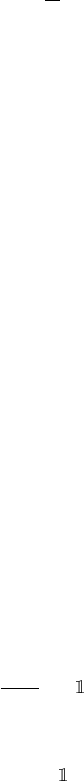
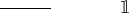
Figure 3.1
Illustration of the projection for the five-location grid used in Example 3.3. The middle
panel depicts the proportion of probability mass assigned to the location
θ
3
= 1 in terms
of the sample return
g
. The left and right panels illustrate this probability assignment at
the boundary locations θ
1
= 0 and θ
m
= 2.
approximate complex distributions using a small, finite set of possible returns.
Under the right conditions, Equation 3.15 gives rise to a convergent algorithm.
The point of convergence of this algorithm is the return function
ˆη
π
(
x
) for which,
for all x ∈X, we have
ˆη
π
(x) = E[Π
c
δ
G
π
(x)
] = E
1 −ζ(G
π
(x))
δ
Π
−
(G
π
(x))
+ ζ(G
π
(x))δ
Π
+
(G
π
(x))
. (3.16)
In fact, we may write
E[Π
c
δ
G
π
(x)
] = Π
c
η
π
(x) ,
where Π
c
η
π
(
x
) denotes distribution supported on
{θ
1
, …, θ
m
}
produced by pro-
jecting each possible outcome under the distribution
η
π
(
x
); we will discuss this
definition in further detail in Chapter 5.
Example 3.3.
Recall the single-state Markov decision process of Example 2.10,
whose return is uniformly distributed on the interval [0
,
2]. Suppose that we take
our support to be the uniform grid
{
0
,
0
.
5
,
1
,
1
.
5
,
2
}
. Let us write
ˆp
0
, ˆp
0.5
, . . . , ˆp
2
for the probabilities assigned to these locations by the projected distribution
ˆη
π
(
x
) = Π
c
η
π
(
x
), where
x
is the unique state of the MDP. The probability density
of the return on the interval [0, 2] is 0.5. We thus have
ˆp
0
(a)
= 0.5
Z
g∈[0,2]
{Π
−
(g) = 0}
(1 −ζ(g)) +
{Π
+
(g) = 0}
ζ(g)
dg
= 0.5
Z
g∈[0,0.5]
(1 −ζ(g))dg
= 0.5
Z
g∈[0,0.5]
(1 −2g)dg
= 0.125.
Draft version.
Learning the Return Distribution 65
In (a), we reexpressed Equation 3.16 in terms of the probability assigned to
ˆp
0
. A similar computation shows that
ˆp
0.5
=
ˆp
1
=
ˆp
1.5
= 0
.
25, while
ˆp
2
= 0
.
125.
Figure 3.1 illustrates the process of assigning probability mass to different
locations. Intuitively, the solution makes sense: there is less probability mass
near the boundaries of the interval [0, 2]. 4
3.6 Categorical Temporal-Difference Learning
With the use of a projection step, the categorical Monte Carlo method allows us
to approximate the return-distribution function of a given policy from sample
trajectories and using a fixed amount of memory. Like the Monte Carlo method
for value functions, however, it ignores the relationship between successive
states in the trajectory. To leverage this relationship, we turn to categorical
temporal-difference learning (CTD).
Consider now a sample transition (
x, a, r, x
0
). Like the categorical Monte
Carlo algorithm, CTD maintains a return function estimate
η
(
x
) supported on
the evenly spaced locations
{θ
1
, . . . , θ
m
}
. Like temporal-difference learning, it
learns by bootstrapping from its current return function estimate. In this case,
however, the update target is a probability distribution supported on
{θ
1
, . . . , θ
m
}
.
The algorithm first constructs an intermediate target by scaling the return
distribution
η
(
x
0
) at the next state by the discount factor
γ
, then shifting it by
the sample reward r. That is, if we write
η(x
0
) =
m
X
i=1
p
i
(x
0
)δ
θ
i
,
then the intermediate target is
˜η(x) =
m
X
i=1
p
i
(x
0
)δ
r+γθ
i
,
which can also be expressed in terms of a pushforward distribution:
˜η(x) = (b
r,γ
)
#
η(x
0
) . (3.17)
Observe that the shifting and scaling operations are applied to each particle
in isolation. After shifting and scaling, however, these particles in general no
longer lie in the support of the original distribution. This motivates the use of the
projection step described in the previous section. Let us denote the intermediate
particles by
˜
θ
i
= b
r,γ
(θ
i
) = r + γθ
i
.
Draft version.

66 Chapter 3
The CTD target is formed by individually projecting each of these particles
back onto the support and combining their probabilities. That is,
Π
c
(b
r,γ
)
#
η(x
0
) =
m
X
j=1
p
j
(x
0
)Π
c
δ
r+γθ
j
.
More explicitly, this is
Π
c
(b
r,γ
)
#
η(x
0
) =
m
X
j=1
p
j
(x
0
)
(1 −ζ(
˜
θ
j
))δ
Π
−
(
˜
θ
j
)
+ ζ(
˜
θ
j
)δ
Π
+
(
˜
θ
j
)
=
m
X
i=1
δ
θ
i
m
X
j=1
p
j
(x
0
)ζ
i, j
(r)
, (3.18)
where
ζ
i, j
(r) =
(1 −ζ(
˜
θ
j
))
{Π
−
(
˜
θ
j
) = θ
i
}
+ ζ(
˜
θ
j
)
{Π
+
(
˜
θ
j
) = θ
i
}
.
In Equation 3.18, the second line highlights that the CTD target is a probability
distribution supported on
{θ
1
, . . . , θ
m
}
. The probabilities assigned to specific
locations are given by the inner sum; as shown here, this assignment is obtained
by weighting the next-state probabilities p
j
(x
0
) by the coefficients ζ
i, j
(r).
The CTD update adjusts the return function estimate
η
(
x
) toward this target:
η(x) ←(1 −α)η(x) + α
Π
c
(b
r,γ
)
#
η(x
0
)
. (3.19)
Expressed in terms of the probabilities of the distributions
η
(
x
) and
η
(
x
0
), this
is (for i = 1, . . . , m)
p
i
(x) ←(1 −α)p
i
(x) + α
m
X
j=1
ζ
i, j
(r)p
j
(x
0
) . (3.20)
With this form, we see that the CTD update rule adjusts each probability
p
i
(
x
)
of the return distribution at state
x
toward a mixture of the probabilities of the
return distribution at the next state (see Algorithm 3.4).
The definition of the intermediate target in pushforward terms (Equation
3.17) illustrates that categorical temporal-difference learning relates to the
distributional Bellman equation
η
π
(x) = E
π
[(b
R,γ
)
#
η
π
(X
0
) |X = x] ,
analogous to the relationship between TD learning and the classical Bellman
equation. We will continue to explore this relationship in later chapters. How-
ever, the two algorithms usually learn different solutions, due to the introduction
of approximation error from the bootstrapping process.
Example 3.4.
We can study the behavior of the categorical temporal-difference
learning algorithm by visualizing how its predictions vary over the course
Draft version.

Learning the Return Distribution 67
Algorithm 3.4: Online categorical temporal-difference learning
Algorithm parameters: step size α ∈(0, 1],
policy π : X→P(A),
evenly spaced locations θ
1
, …, θ
m
∈R,
initial probabilities
(p
0
i
(x))
H
i=0
: x ∈X
(p
i
(x))
H
i=0
←(p
0
i
(x))
H
i=0
for all x ∈X
Loop for each episode:
Observe initial state x
0
Loop for t = 0, 1, . . .
Draw a
t
from π( · | x
t
)
Take action a
t
, observe r
t
, x
t+1
ˆp
i
←0 for i = 1, …, m
for j = 1, …, m do
if x
t+1
is terminal then
g ←r
t
else
g ←r
t
+ γθ
j
if g ≤θ
1
then
ˆp
1
← ˆp
1
+ p
j
(x
t+1
)
else if g ≥θ
m
then
ˆp
m
← ˆp
m
+ p
j
(x
t+1
)
else
i
∗
← largest i s.t. θ
i
≤g
ζ ←
g−θ
i
∗
θ
i
∗
+1
−θ
i
∗
ˆp
i
∗
← ˆp
i
∗
+ (1 −ζ)p
j
(x
t+1
)
ˆp
i
∗
+1
← ˆp
i
∗
+1
+ ζp
j
(x
t+1
)
end for
for i = 1, …, m do
p
i
(x
t
) ←(1 −α)p
i
(x
t
) + α ˆp
i
end for
until x
t+1
is terminal
end
of learning. We apply CTD to approximate the return function of the safe
policy in the Cliffs domain (Example 2.9). Learning takes place online (as per
Algorithm 3.4), using a constant step size of
α
= 0
.
05, and return distributions
are approximated with m = 31 locations evenly spaced between −1 and 1.
Draft version.
68 Chapter 3
1.0 0.5 0.0 0.5 1.0
0.00
0.25
0.50
0.75
1.00
Probability
Return
Probability
Return
Probability
Return
Probability
Return
1.0 0.5 0.0 0.5 1.0
0.00
0.05
0.10
0.15
Probability
Return
1.0 0.5 0.0 0.5 1.0
0.00
0.05
0.10
0.15
Probability
Return
1.0 0.5 0.0 0.5 1.0
0.00
0.05
0.10
0.15
Probability
Return
1.0 0.5 0.0 0.5 1.0
0.00
0.05
0.10
0.15
Probability
Return
1.0 0.5 0.0 0.5 1.0
0.0
0.1
0.2
0.3
0.4
0.5
1.0 0.5 0.0 0.5 1.0
0.00
0.05
0.10
0.15
Probability
Return
1.0 0.5 0.0 0.5 1.0
0.00
0.05
0.10
0.15
Probability
Return
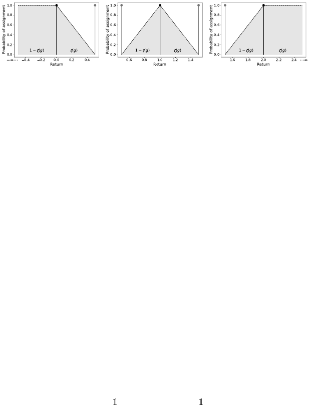
Figure 3.2
The return distribution at the initial state in the Cliffs domain, as predicted by categorical
temporal-difference learning over the course of learning.
Top panels.
The predictions
after
e ∈{
0
,
1000
,
2000
,
10000
}
episodes (
α
= 0
.
05; see Algorithm 3.4). Here, the return
distributions are initialized by assigning equal probability to all locations.
Bottom pan-
els.
Corresponding predictions when the return distributions initially put all probability
mass on the zero return.
(a) (b) (c)
1.0 0.5 0.0 0.5 1.0
Return
0
2
4
6
8
10
Density
1.0 0.5 0.0 0.5 1.0
Return
0.0
0.1
0.2
0.3
0.4
0.5
Probability
1.0 0.5 0.0 0.5 1.0
Return
0.00
0.05
0.10
0.15
0.20
0.25
Probability
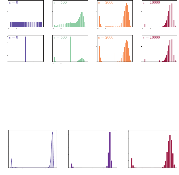
Figure 3.3
(a)
The return distribution at the initial state in the Cliffs domain, visualized using
kernel density estimation (see Figure 2.2).
(b)
The return-distribution estimate learned
by the categorical Monte Carlo algorithm with
m
= 31.
(c)
The estimate learned by the
categorical temporal-difference learning algorithm.
Figure 3.2 illustrates that the initial return function plays a substantial role in
the speed at which CTD learns a good approximation. Informally, this occurs
because the uniform distribution is closer to the final approximation than the
distribution that puts all of its probability mass on zero (what “close” means in
this context will be the topic of Chapter 4). In addition, we see that categorical
temporal-difference learning learns a different approximation to the true return
function, compared to the categorical Monte Carlo algorithm (Figure 3.3). This
is due to a phenomenon we call diffusion, which arises from the combination of
the bootstrapping step and projection; we will study diffusion in Chapter 5.
4
Draft version.
Learning the Return Distribution 69
3.7 Learning to Control
A large part of this book considers the problem of learning to predict the dis-
tribution of an agent’s returns. In Chapter 7, we will discuss how one might
instead learn to maximize or control these returns and the role that distribu-
tional reinforcement learning plays in this endeavor. By learning to control, we
classically mean obtaining (from experience) a policy
π
∗
that maximizes the
expected return:
E
π
∗
h
∞
X
t=0
γ
t
R
t
i
≥E
π
h
∞
X
t=0
γ
t
R
t
i
, for all π .
Such a policy is called an optimal policy. From Section 2.5, recall that the
state-action value function Q
π
is given by
Q
π
(x, a) = E
π
h
∞
X
t=0
γ
t
R
t
X
0
= x, A
0
= a
i
.
Any optimal policy π
∗
has the property that its state-action value function also
satisfies the Bellman optimality equation:
Q
π
∗
(x, a) = E
π
R + γ max
a
0
∈A
Q
π
∗
(X
0
, a
0
) |X = x, A = a
.
Similar in spirit to temporal-difference learning, Q-learning is an incremental
algorithm that finds an optimal policy. Q-learning maintains a state-action value
function estimate, Q, which it updates according to
Q(x, a) ←(1 −α)Q(x, a) + α
r + γ max
a
0
∈A
Q(x
0
, a
0
)
. (3.21)
The use of the maximum in the Q-learning update rule results in different
behavior than TD learning, as the selected action depends on the current value
estimate. We can think of this difference as constructing one target for each
action
a
0
and updating the value estimate toward the largest of such targets.
It can be shown that under the right conditions, Q-learning converges to the
optimal state-action value function
Q
∗
, corresponding to the expected return
under any optimal policy. We extract an optimal policy from
Q
∗
by acting
greedily with respect to
Q
∗
: that is, choosing a policy
π
∗
that selects maximally
valued actions according to Q
∗
.
The simplest way to extend Q-learning to the distributional setting is to
express the maximal action in Equation 3.21 as a greedy policy. Denote by
η
a return-function estimate over state-action pairs, such that
η
(
x, a
) is the
return distribution associated with the state-action pair (
x, a
)
∈X×A
. Define
the greedy action
a
η
(x) = arg max
a∈A
E
Z∼η(x,a)
[Z] ,
Draft version.

70 Chapter 3
breaking ties arbitrarily. The categorical Q-learning update rule is
η(x, a) ←(1 −α)η(x, a) + α
Π
c
(b
r,γ
)
#
η
x
0
, a
η
(x
0
)
.
It can be shown that, under the same conditions as Q-learning, the mean of the
return-function estimates also converges to
Q
∗
. The behavior of the distributions
themselves, however, may be surprisingly complicated. We can also put the
learned distributions to good use and make decisions on the basis of their
full characterization, rather than from their mean alone. This forms the topic
of risk-sensitive reinforcement learning. We return to both of these points in
Chapter 7.
3.8 Further Considerations
Categorical temporal-difference learning learns to predict return distributions
from sample experience. As we will see in subsequent chapters, the choices that
we made in designing CTD are not unique, and the algorithm is best thought of
as a jumping-off point into a broad space of methods. For example, an important
question in distributional reinforcement learning asks how we should represent
probability distributions, given a finite memory budget. One issue with the
categorical representation is that it relies on a fixed grid of locations to cover the
range [
θ
1
, θ
m
], which lacks flexibility and is in many situations inefficient. We
will take a closer look at this issue in Chapter 5. In many practical situations,
we also need to deal with a few additional considerations, including the use of
function approximation to deal with very large state spaces (Chapters 9 and 10).
3.9 Technical Remarks
Remark 3.1
(Nonparametric distributional Monte Carlo algorithm)
.
In
Section 3.4, we saw that the (unprojected) finite-horizon categorical Monte
Carlo algorithm can in theory learn finite-horizon return-distribution functions
when there are only a small number of possible returns. It is possible to extend
these ideas to obtain a straightforward, general-purpose algorithm that can be
sometimes be used to learn an accurate approximation to the return distribution.
Like the sample-mean Monte Carlo method, the nonparametric distributional
Monte Carlo algorithm takes as input
K
finite-length trajectories with a com-
mon source state
x
0
. After computing the sample returns (
g
k
)
K
k=1
from these
trajectories, it constructs the estimate
ˆη
π
(x
0
) =
1
K
K
X
k=1
δ
g
k
(3.22)
of the return distribution
η
π
(
x
0
). Here, nonparametric refers to the fact that
the approximating distribution in Equation 3.22 is not described by a finite
Draft version.
Learning the Return Distribution 71
collection of parameters; in fact, the memory required to represent this object
may grow linearly with
K
. Although this is not an issue when
K
is relatively
small, this can be undesirable when working with large amounts of data and
moreover precludes the use of function approximation (see Chapters 9 and 10).
However, unlike the categorical Monte Carlo and temporal-difference learn-
ing algorithms presented in this chapter, the accuracy of this estimate is only
limited by the number of trajectories
K
; we describe various ways to quantify
this accuracy in Remark 4.3. As such, it provides a useful baseline for measuring
the quality of other distributional algorithms. In particular, we used this algo-
rithm to generate the ground-truth return-distribution estimates in Example 2.9
and in Figure 3.3. 4
3.10 Bibliographical Remarks
The development of a distributional algorithm in this chapter follows our own
development of the distributional perspective, beginning with our work on using
compression algorithms in reinforcement learning (Veness et al. 2015).
3.1.
The first-visit Monte Carlo estimate is studied by Singh and Sutton (1996),
where it is used to characterize the properties of replacing eligibility traces (see
also Sutton and Barto 2018). Statistical properties of model-based estimates
(which solve for the Markov decision process’s parameters as an intermediate
step) are analyzed by Mannor et al. (2007). Grünewälder and Obermayer (2011)
argue that model-based methods must incur statistical bias, an argument that
also extends to temporal-difference algorithms. Their work also introduces a
refined sample-mean Monte Carlo method that yields a minimum-variance
unbiased estimator (MVUE) of the value function. See Browne et al. (2012) for
a survey of Monte Carlo tree search methods and Liu (2001), Robert and Casella
(2004), and Owen (2013) for further background on Monte Carlo methods more
generally.
3.2.
Incremental algorithms are a staple of reinforcement learning and have
roots in stochastic approximation (Robbins and Monro 1951; Widrow and Hoff
1960; Kushner and Yin 2003) and psychology (Rescorla and Wagner 1972). In
the control setting, these are also called optimistic policy iteration methods and
exhibit fairly complex behavior (Sutton 1999; Tsitsiklis 2002).
3.3.
Temporal-difference learning was introduced by Sutton (1984, 1988). The
sample transition model presented here differs from the standard algorithmic
presentation but allows us to separate concerns of behavior (data collection)
from learning. A similar model is used in Bertsekas and Tsitsiklis (1996) to
prove convergence of a broad class of TD methods and by Azar et al. (2012) to
provide sample efficiency bounds for model-based control.
Draft version.

72 Chapter 3
3.4.
What is effectively the undiscounted finite-horizon categorical Monte Carlo
algorithm was proposed by Veness et al. (2015). There, the authors demonstrate
that by means of Bayes’s rule, one can learn the return distribution by first
learning the joint distribution over returns and states (in our notation,
P
π
(
X, G
))
by means of a compression algorithm and subsequently using Bayes’s rule
to extract
P
π
(
G | X
). The method proved surprisingly effective at learning to
play Atari 2600 games. Toussaint and Storkey (2006) consider the problem of
control as probabilistic inference, where the reward and trajectory length are
viewed as random variables to be optimized over, again obviating the need to
deal with a potentially large support for the return.
3.5–3.6.
Categorical temporal-difference learning for both prediction and
control was introduced by Bellemare et al. (2017a), in part to address the
shortcomings of the undiscounted algorithm. Its original form contains both the
projection step and the categorical representation as given here. The mixture
update that we study in this chapter is due to Rowland et al. (2018).
3.7.
The Q-learning algorithm is due to Watkins (1989); see also Watkins and
Dayan (1992). The explicit construction of a greedy policy is commonly found
in more complex reinforcement learning algorithms, including modified policy
iteration (Puterman and Shin 1978),
λ
-policy iteration (Bertsekas and Ioffe
1996), and nonstationary policy iteration (Scherrer and Lesner 2012; Scherrer
2014).
3.9.
The algorithm introduced in Remark 3.1 is essentially an application of the
standard Monte Carlo method to the return distribution and is a special case of
the framework set out by Chandak et al. (2021), who also analyze the statistical
properties of the approach.
3.11 Exercises
Exercise 3.1.
Suppose that we begin with the initial value function estimate
V(x) = 0 for all x ∈X.
(i)
Consider first the setting in which we are given sample returns for a single
state
x
. Show that in this case, the incremental Monte Carlo algorithm
(Equation 3.6), instantiated with
α
k
=
1
k+1
, is equivalent to computing the
sample-mean Monte Carlo estimate for
x
. That is, after processing the
sample returns g
1
, . . . , g
K
, we have
V
K
(x) =
1
K
K
X
i=1
g
i
.
(ii)
Now consider the case where source states are drawn from a distribution
ξ
, with
ξ
(
x
)
>
0 for all
x
, and let
N
k
(
x
k
) be the number of times
x
k
has been
Draft version.

Learning the Return Distribution 73
updated up to but excluding time
k
. Show that the appropriate step size to
match the sample-mean Monte Carlo estimate is α
k
=
1
N
k
(x
k
)+1
. 4
Exercise 3.2. Recall from Exercise 2.8 the n-step Bellman equation:
V
π
(x) = E
π
h
n−1
X
t=0
γ
t
R
t
+ γ
n
V
π
(X
n
) | X
0
= x
.
Explain what a sensible
n
-step temporal-difference learning update rule might
look like. 4
Exercise 3.3.
The Cart–Pole domain is a small, two-dimensional reinforcement
learning problem (Barto et al. 1983). In this problem, the learning agent must
balance a swinging pole that is a attached to a moving cart. Using an open-
source implementation of Cart–Pole, implement the undiscounted finite-horizon
categorical Monte Carlo algorithm and evaluate its behavior. Construct a finite
state space by discretising the four-dimensional state space using a uniform grid
of size 10
×
10
×
10
×
10. Plot the learned return distribution for a fixed initial
state and other states of your choice when
(i) the policy chooses actions uniformly at random;
(ii)
the policy moves the cart in the direction that the pole is leaning toward.
4
You may want to pick the horizon H to be the maximum length of an episode.
Exercise 3.4.
Implement the categorical Monte Carlo (CMC), nonparametric
categorical Monte Carlo (Remark 3.1), and categorical temporal-difference
learning (CTD) algorithms. For a discount factor
γ
= 0
.
99, compare the return
distributions learned by these three algorithms on the Cart–Pole domain of the
previous exercise. For CMC and CTD, vary the number of particles
m
and the
range of the support [
θ
1
, θ
m
]. How do the approximations vary as a function of
these parameters? 4
Exercise 3.5.
Suppose that the rewards
R
t
take on one of
N
R
values. Consider
the undiscounted finite-horizon return
G =
H−1
X
t=0
R
t
.
Denote by N
G
the number of possible realizations of G.
(i) Show that N
G
can be as large as
N
R
+H−1
H
.
(ii) Derive a better bound when R
t
∈{0, 1, . . . , N
R
−1}.
(iii)
Explain, in words, why the bound is better in this case. Are there other sets
of rewards for which N
G
is smaller than the worst-case from (i)? 4
Draft version.

74 Chapter 3
Exercise 3.6.
Recall from Section 3.5 that the categorical Monte Carlo
algorithm aims to find the approximation
ˆη
π
m
(x) = Π
c
η
π
(x), x ∈X,
where we use the subscript
m
to more explicitly indicate that the quality of this
approximation depends on the number of locations.
Consider again the problem setting of Example 3.3. For
m ≥
2, suppose that
we take θ
1
= 0 and θ
m
= 2, such that
θ
i
= 2
i −1
m −1
i = 1, . . . m .
Show that in this case,
ˆη
π
m
(
x
) converges to the uniform distribution on the
interval [0, 2], in the sense that
lim
m→∞
ˆη
π
m
(x)
[a, b]
→
b −a
2
for all
a < b
; recall that
ν
([
a, b
]) denotes the probability assigned to the interval
[a, b] by a probability distribution ν. 4
Exercise 3.7.
The purpose of this exercise is to demonstrate that the categorical
Monte Carlo algorithm is what we call mean-preserving. Consider a sequence
of state-return pairs (
x
k
, g
k
)
K
k=1
and an evenly spaced grid
{θ
1
, . . . , θ
m
}
,
m ≥
2.
Suppose that rewards are bounded in [R
min
, R
max
].
(i)
Suppose that
V
min
≥θ
1
and
V
max
≤θ
m
. For a given
g ∈
[
V
min
, V
max
], show that
the distribution ν = Π
c
δ
g
satisfies
E
Z∼ν
[Z] = g .
(ii)
Based on this, argue that if
η
(
x
) is a distribution with mean
V
, then after
applying the update
η(x) ←(1 −α)η(x) + αΠ
c
δ
g
,
the mean of η(x) is (1 −α)V + αg.
(iii)
By comparing with the incremental Monte Carlo update rule, explain why
categorical Monte Carlo can be said to be mean-preserving.
(iv)
Now suppose that [
V
min
, V
max
]
*
[
θ
1
, θ
m
]. How are the preceding results
affected? 4
Exercise 3.8.
Following the notation of Section 3.5, consider the nearest
neighbor projection method
Π
nn
g =
(
Π
−
(g) if ζ(g) ≤0.5
Π
+
(g) otherwise.
Draft version.
Learning the Return Distribution 75
Show that this projection is not mean-preserving in the sense of the preceding
exercise. Implement and evaluate on the Cart–Pole domain. What do you
observe? 4
Draft version.