2
The Distribution of Returns
Training for a marathon. Growing a vegetable garden. Working toward a piano
recital. Many of life’s activities involve making decisions whose benefits are
realized only later in the future (whether to run on a particular Saturday morning;
whether to add fertilizer to the soil). In reinforcement learning, these benefits
are summarized by the return received following these decisions. The return is a
random quantity that describes the sum total of the consequences of a particular
activity – measured in dollars, points, bits, kilograms, kilometers, or praise.
Distributional reinforcement learning studies the random return. It asks ques-
tions such as: How should it be described, or approximated? How can it be
predicted on the basis of past observations? The overarching aim of this book
is to establish a language with which such questions can be answered. By
virtue of its subject matter, this language is somewhere at the intersection of
probability theory, statistics, operations research, and of course reinforcement
learning itself. In this chapter, we begin by studying how the random return
arises from sequential interactions and immediate rewards. From this, we estab-
lish the fundamental relationship of random returns: the distributional Bellman
equation.
2.1 Random Variables and Their Probability Distributions
A quantity that we wish to model as random can be represented via a random
variable. For example, the outcome of a coin toss can be represented with a
random variable, which may take on either the value “heads” or “tails”. We
can reason about a random variable through its probability distribution, which
specifies the probability of its possible realizations.
Example 2.1.
Consider driving along a country road toward a railway crossing.
There are two possible states that the crossing may be in. The crossing may
be open, in which case you can drive straight through, or it may be closed,
in which case you must wait for the train to pass and for the barriers to lift
Draft version. 11

12 Chapter 2
before driving on. We can model the state of the crossing as a random variable
C
with two outcomes, “open” and “closed.” The distribution of
C
is specified
by a probability mass function, which provides the probability of each possible
outcome:
P(C = “open”) = p , P(C = “closed”) = 1 − p ,
for some p ∈[0, 1]. 4
Example 2.2.
Suppose we arrive at the crossing described above and the barri-
ers are down. We may model the waiting time
T
(in minutes) until the barriers
are open again as a uniform distribution on the interval [0
,
10]; informally,
any real value between 0 and 10 is equally likely. In this case, the probability
distribution can be specified through a probability density function, a function
f
:
R →
[0
, ∞
). In the case of the uniform distribution above, this function is
given by
f (t) =
1
10
if t ∈[0, 10]
0 otherwise
.
The density then provides the probability of
T
lying in any interval [
a, b
]
according to
P(T ∈[a, b]) =
Z
b
a
f (t)dt . 4
In this book, we will encounter instances of random variables – such as
rewards and returns – that are discrete, have densities, or in some cases fall in
neither category. To deal with this heterogeneity, one solution is to describe
probability distributions over
R
using their cumulative distribution function
(CDF), which always exists. The cumulative distribution function associated
with a random variable Z is the function F
Z
: R →[0, 1] defined by
F
Z
(z) = P(Z ≤z) .
In distributional reinforcement learning, common operations on random
variables include summation, multiplication by a scalar, and indexing into col-
lections of random variables. Later in the chapter, we will see how to describe
these operations in terms of cumulative distribution functions.
Example 2.3.
Suppose that now we consider the random variable
T
0
describing
the total waiting time experienced at the railroad crossing. If we arrive at the
crossing and it is open (
C
=
“open”
), there is no need to wait and
T
0
= 0. If,
however, the barrier is closed (
C
=
“closed”
), the waiting time is distributed
Draft version.

The Distribution of Returns 13
uniformly on [0, 10]. The cumulative distribution function of T
0
is
F
T
0
(t) =
0 t < 0
p t = 0
p +
(1−p)t
10
0 < t < 10
1 t ≥10 .
Observe that there is a nonzero probability of
T
0
taking the value 0 (which
occurs when the crossing is open), so the distribution cannot have a density. Nor
can it have a probability mass function, as there are a continuum of possible
waiting times from 0 to 10 minutes. 4
Another solution is to treat probability distributions atomically, as elements of
the space
P
(
R
) of probability distributions. In this book we favor this approach
over the use of cumulative distribution functions, as it lets us concisely express
operations on probability distributions. The probability distribution that puts
all of its mass on
z ∈R
, for example, is the Dirac delta denoted
δ
z
; the uniform
distribution on the interval from
a
to
b
is
U
([
a, b
]). Both distributions belong to
P
(
R
). The distribution of the random variable
T
0
in Example 2.3 also belongs
to
P
(
R
). It is a mixture of distributions and can be written in terms of its
constituent parts:
pδ
0
+ (1 − p)U([0, 10]) .
More formally, these objects are probability measures: functions that associate
different subsets of outcomes with their respective probabilities. If
Z
is a real-
valued random variable and
ν
is its distribution, then for a subset
S ⊆R
,
3
we
write
ν(S ) = P(Z ∈S ) .
In particular, the probability assigned to
S
by a mixture distribution is the
weighted sum of probabilities assigned by its constituent parts: for
ν
1
, ν
2
∈P
(
R
)
and p ∈[0, 1], we have
pν
1
+ (1 − p)ν
2
(S ) = pν
1
(S ) + (1 − p)ν
2
(S ) .
With this language, the cumulative distribution function of
ν ∈P
(
R
) can be
expressed as
F
ν
(y) = ν((−∞, y]) .
This notation also extends to distributions over outcomes that are not real-valued.
For instance, P({“open”, “closed”}) is the set of probability distributions over
the state of the railroad crossing in Example 2.1. Probability distributions (as
3. Readers expecting to see the qualifier “measurable” here should consult Remark 2.1.
Draft version.
14 Chapter 2
Agent
Environment
action
state reward
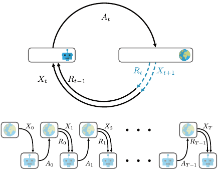
Figure 2.1
Top:
The Markov decision process model of the agent’s interactions with its environment.
Bottom:
The same interactions, unrolled to show the sequence of random variables
(X
t
, A
t
, R
t
)
t≥0
, beginning at time t = 0 and up to the state X
T
.
elements of
P
(
R
)) make it possible to express some operations on distributions
that would be unwieldy to describe in terms of random variables.
2.2 Markov Decision Processes
In reinforcement learning, an environment is any of a wide variety of systems
that emit observations, can be influenced, and persist in one form or another
over time. A data center cooling system, a remote-controlled helicopter, a stock
market, and a video game console can all be thought of as environments. An
agent interacts with its environment by making choices that have consequences
in this environment. These choices may be implemented simply as an if state-
ment in a simulator or they may require a human to perform some task in our
physical world.
We assume that interactions take place or are recorded at discrete time
intervals. These give rise to a sequential process in which at any given time
t ∈N
=
{
0
,
1
,
2
, …}
, the current situation is described by a state
X
t
from a finite
set
X
.
4
The initial state is a random variable
X
0
with probability distribution
ξ
0
∈P (X).
4.
Things tend to become more complicated when one considers infinite state spaces; see
Remark 2.3.
Draft version.
The Distribution of Returns 15
The agent influences its future by choosing an action
A
t
from a finite set of
actions
A
. In response to this choice, the agent is provided with a real-valued
reward
R
t
.
5
This reward indicates to the agent the usefulness or worth of its
choice. The action also affects the state of the system; the new state is denoted
X
t+1
. An illustration of this sequential interaction is given in Figure 2.1. The
reward and next state are modeled by the transition dynamics
P
:
X×A→
P
(
R ×X
) of the environment, which provides the joint probability distribution
of
R
t
and
X
t+1
in terms of the state
X
t
and action
A
t
. We say that
R
t
and
X
t+1
are
drawn from this distribution:
R
t
, X
t+1
∼P(·, · | X
t
, A
t
) . (2.1)
In particular, when R
t
is discrete, Equation 2.1 can be directly interpreted as
P(R
t
= r, X
t+1
= x
0
| X
t
= x, A
t
= a) = P(r, x
0
| x, a).
Modeling the two quantities jointly is useful in problems where the reward
depends on the next state (common in board games, where the reward is asso-
ciated with reaching a certain state) or when the state depends on the reward
(common in domains where the state keeps track of past rewards). In this book,
however, unless otherwise noted, we make the simplifying assumption that
the reward and next state are independent given
X
t
and
A
t
, and separate the
transition dynamics into a reward distribution and transition kernel:
R
t
∼P
R
(· | X
t
, A
t
)
X
t+1
∼P
X
(· | X
t
, A
t
) .
A Markov decision process (MDP) is a tuple (
X, A, ξ
0
, P
X
, P
R
) that contains
all the information needed to describe how the agent’s decisions influence
its environment. These decisions are not themselves part of the model but
instead arise from a policy. A policy is a mapping
π
:
X→P
(
A
) from states to
probability distributions over actions such that
A
t
∼π(· | X
t
) .
Such policies choose the action
A
t
solely on the basis of the immediately
preceding state
X
t
and possibly a random draw. Technically, these are a special
subset of decision-making rules that are both stationary (they do not depend
on the time
t
at which the decision is to be taken, except through the state
X
t
)
and Markov (they do not depend on events prior to time
t
). Stationary Markov
policies will be enough for us for most of this book, but we will study more
general policies in Chapter 7.
5.
An alternative convention is to denote the reward that follows action
A
t
by
R
t+1
. Here we prefer
R
t
to emphasize the association between action and reward.
Draft version.
16 Chapter 2
Finally, a state
x
∅
from which no other states can be reached is called
absorbing or terminal. For all actions a ∈A, its next-state distribution is
P
X
(x
∅
| x
∅
, a) = 1.
Terminal states correspond to situations in which further interactions are irrele-
vant: once a game of chess is won by one of the players, for example, or once a
robot has successfully accomplished a desired task.
2.3 The Pinball Model
The game of American pinball provides a useful metaphor for how the various
pieces of a Markov decision process come together to describe real systems.
A classic American pinball machine consists of a slanted, glass-enclosed play
area filled with bumpers of various shapes and sizes. The player initiates the
game by using a retractable spring to launch a metal ball into the play area, a
process that can be likened to sampling from the initial state distribution. The
metal ball progresses through the play area by bouncing off the various bumpers
(the transition function), which reward the player with a variable number of
points (the reward function). The game ends when the ball escapes through a
gap at the bottom of the play area, to which it is drawn by gravity (the terminal
state). The player can prevent this fate by controlling the ball’s course with
a pair of flippers on either side of the gap (the action space). Good players
also use the flippers to aim the ball toward the most valuable bumpers or other,
special high-scoring zones and may even physically shake the pinball cabinet
(called nudging) to exert additional control. The game’s state space describes
possible arrangements of the machine’s different moving parts, including the
ball’s location.
Turning things around, we may think of any Markov decision process as an
abstract pinball machine. Initiated by the equivalent of inserting the traditional
quarter into the machine, we call a single play through the Markov decision
process a trajectory, beginning from the random initial state and lasting until a
terminal state is reached. This trajectory is the sequence
X
0
, A
0
, R
0
, X
1
, A
1
, . . .
of random interleaved states, actions, and rewards. We use the notation
(X
t
, A
t
, R
t
)
t≥0
to express this sequence compactly.
The various elements of the trajectory depend on each other according to the
rules set by the Markov decision process. These rules can be summarized by a
collection of generative equations, which tell us how we might write a program
for sampling a trajectory one variable at a time. For a time step
t ∈N
, let us
denote by
X
0:t
,
A
0:t
, and
R
0:t
the subsequences (
X
0
, X
1
, . . . , X
t
), (
A
0
, A
1
, . . . , A
t
),
Draft version.

The Distribution of Returns 17
and (R
0
, R
1
, . . . , R
t
), respectively. The generative equations are
X
0
∼ξ
0
;
A
t
|(X
0:t
, A
0:t−1
, R
0:t−1
) ∼π( ·|X
t
), for all t ≥0 ;
R
t
|(X
0:t
, A
0:t
, R
0:t−1
) ∼P
R
(·|X
t
, A
t
), for all t ≥0 ;
X
t+1
|(X
0:t
, A
0:t
, R
0:t
) ∼P
X
( · | X
t
, A
t
), for all t ≥0 .
We use the notation
Y |
(
Z
0
, Z
1
, . . .
) to indicate the basic dependency structure
between these variables. The equation for
A
t
, for example, is to be interpreted
as
P
A
t
= a | X
0
, A
0
, R
0
, ··· , X
t−1
, A
t−1
, R
t−1
, X
t
) = π(a | X
t
.
For
t
= 0, the notation
A
0:t−1
and
R
0:t−1
denotes the empty sequence. Because
the policy fixes the “decision” part of the Markov decision process formalism,
the trajectory can be viewed as a Markov chain over the space
X×A×R
. This
model is sometimes called a Markov reward process.
By convention, terminal states yield no reward. In these situations, it is
sensible to end the sequence at the time
T ∈N
at which a terminal state is first
encountered. It is also common to notify the agent that a terminal state has
been reached. In other cases (such as Example 2.4 below), the sequence might
(theoretically) go on forever.
We use the notion of a joint distribution to formally ask questions (and
give answers) about the random trajectory. This is the joint distribution over
all random variables involved, denoted
P
π
(
·
). For example, the probability
that the agent begins in state
x
and finds itself in that state again after
t
time
steps when acting according to a policy
π
can be mathematically expressed
as
P
π
(
X
0
=
x, X
t
=
x
). Similarly, the probability that a positive reward will be
received at some point in time is
P
π
(there exists t ≥0 such that R
t
> 0) .
The explicit policy subscript is a convention to emphasize that the agent’s
choices affect the distribution of outcomes. It also lets us distinguish statements
about random variables derived from the random trajectory from statements
about other, arbitrary random variables.
The joint distribution
P
π
gives rise to the expectation
E
π
over real-valued
random variables. This allows us to write statements such as
E
π
[2 ×R
0
+
{X
1
= X
0
}
R
1
] .
Remark 2.1 provides additional technical details on how this expectation can be
constructed from P
π
.
Draft version.
18 Chapter 2
Example 2.4.
The martingale is a betting strategy popular in the eighteenth
century and based on the principle of doubling one’s ante until a profit is made.
This strategy is formalized as a Markov decision process where the (infinite)
state space
X
=
Z
is the gambler’s loss thus far, with negative losses denoting
gains. The action space
A
=
N
is the gambler’s bet.
6
If the game is fair, then for
each state x and each action a,
P
X
(x + a | x, a) = P
X
(x −a | x, a) =
1
/2.
Placing no bet corresponds to
a
= 0. With
X
0
= 0, the martingale policy is
A
0
= 1
and for t > 0,
A
t
=
(
X
t
+ 1 X
t
> 0
0 otherwise.
Formally speaking, the policy maps each loss
x >
0 to
δ
x+1
, the Dirac distribution
at
x
+ 1, and all negative states (gains) to
δ
0
. Simple algebra shows that for
t >
0,
X
t
=
(
2
t
−1 with probability 2
−t
,
−1 with probability 1 −2
−t
.
That is, the gambler is assured to eventually make a profit (since 2
−t
→
0), but
arbitrary losses may be incurred before a positive gain is made. Calculations
show that the martingale strategy has nil expected gain (
E
π
[
X
t
] = 0 for
t ≥
0), while the variance of the loss grows unboundedly with the number of
rounds played (
E
π
[
X
2
t
]
→∞
); as a result, it is frowned upon in many gambling
establishments. 4
The notation
P
π
makes clear the dependence of the distribution of the random
trajectory (
X
t
, A
t
, R
t
)
t≥0
on the agent’s policy
π
. Often, we find it also useful
to view the initial state distribution
ξ
0
as a parameter to be reasoned explicitly
about. In this case, it makes sense to more explicitly denote the joint distribution
by
P
ξ
0
,π
. The most common situation is when we consider the same Markov
decision process but initialized at a specific starting state
x
. In this case, the
distribution becomes
ξ
0
=
δ
x
, meaning that
P
ξ
0
,π
(
X
0
=
x
) = 1. We then use the
fairly standard shorthand
P
π
( ·|X
0
= x) = P
δ
x
,π
( · ) , E
π
[ ·|X
0
= x] = E
δ
x
,π
[ · ] .
Technically, this use of the conditioning bar is an abuse of notation. We are
directly modifying the probability distributions of these random variables, rather
than conditioning on an event as the notation normally signifies.
7
However,
this notation is convenient and common throughout the reinforcement learning
6. We are ignoring cash flow issues here.
7.
If we attempt to use the actual conditional probability distribution instead, we find that it is
ill-defined when ξ
0
(x) = 0. See Exercise 2.2.
Draft version.

The Distribution of Returns 19
literature, and we therefore adopt it as well. It is also convenient to modify the
distribution of the first action
A
0
, so that rather than this random variable being
sampled from
π
(
· | X
0
), it is fixed at some action
a ∈A
. We use similar notation
as above to signify the resulting distribution over trajectories and corresponding
expectations:
P
π
( ·|X
0
= x, A
0
= a) , E
π
[ ·|X
0
= x, A
0
= a] .
2.4 The Return
Given a discount factor
γ ∈
[0
,
1), the discounted return
8
(or simply the return)
is the sum of rewards received by the agent from the initial state onward,
discounted according to their time of occurrence:
G =
∞
X
t=0
γ
t
R
t
. (2.2)
The return is a sum of scaled, real-valued random variables and is therefore
itself a random variable. In reinforcement learning, the success of an agent’s
decisions is measured in terms of the return that it achieves: greater returns are
better. Because it is the measure of success, the return is the fundamental object
of reinforcement learning.
The discount factor encodes a preference to receive rewards sooner than
later. In settings that lack a terminal state, the discount factor is also used to
guarantee that the return
G
exists and is finite. This is easily seen when rewards
are bounded on the interval [R
min
, R
max
], in which case we have
G ∈
"
R
min
1 −γ
,
R
max
1 −γ
#
. (2.3)
Throughout this book, we will often write
V
min
and
V
max
for the endpoints of the
interval above, denoting the smallest and largest return obtainable when rewards
are bounded on [
R
min
, R
max
]. When rewards are not bounded, the existence of
G
is still guaranteed under the mild assumption that rewards have finite first
moment; we therefore adopt this assumption throughout the book.
Assumption 2.5.
For each state
x ∈X
and action
a ∈A
, the reward distribution
P
R
( · | x, a) has finite first moment. That is, if R ∼ P
R
( · | x, a), then
E
|R|
< ∞. 4
8.
In parts of this book, we also consider the undiscounted return
P
∞
t=0
R
t
. We sometimes write
γ
= 1 to denote this return, indicating a change from the usual setting. One should be mindful that
we then need to make sure that the sum of rewards converges.
Draft version.

20 Chapter 2
Proposition 2.6.
Under Assumption 2.5, the random return
G
exists and
is finite with probability 1, in the sense that
P
π
G ∈(−∞, ∞)
= 1 . 4
In the usual treatment of reinforcement learning, Assumption 2.5 is taken
for granted (there is little to be predicted otherwise). We still find Proposition
2.6 useful as it establishes that the assumption is sufficient to guarantee the
finiteness of
G
and hence the existence of its probability distribution. The phrase
“with probability 1” allows for the fact that in some realizations of the random
trajectory,
G
is infinite (for example, if the rewards are normally distributed) –
but the probability of observing such a realization is nil. Remark 2.2 gives
more details on this topic, along with a proof of Proposition 2.6; see also
Exercise 2.17.
We call the probability distribution of
G
the return distribution. The return
distribution determines quantities such as the expected return
E
π
G
= E
π
h
∞
X
t=0
γ
t
R
t
i
,
which plays a central role in reinforcement learning, the variance of the return
Var
π
G
= E
π
(G −E
π
[G])
2
,
and tail probabilities such as
P
π
∞
X
t=0
γ
t
R
t
≥0
,
which arise in risk-sensitive control problems (discussed in Chapter 7). As the
following examples illustrate, the probability distributions of random returns
vary from simple to intricate, according to the complexity of interactions
between the agent and its environment.
Example 2.7
(
Blackjack
)
.
The card game of blackjack is won by drawing
cards whose total value is greater than that of a dealer, who plays according to
a known, fixed set of rules. Face cards count for 10, while aces may be counted
as either 1 or 11, to the player’s preference. The game begins with the player
receiving two cards, which they can complement by hitting (i.e., requesting
another card). The game is lost immediately if the player’s total goes over 21,
called going bust. A player satisfied with their cards may instead stick, at which
point the dealer adds cards to their own hand, until a total of 17 or more is
reached.
Draft version.

The Distribution of Returns 21
If the player’s total is greater than the dealer’s or the dealer goes bust, they
are paid out their ante; otherwise, the ante is lost. In the event of a tie, the player
keeps the ante. We formalize this as receiving a reward of 1,
−
1, or 0 when play
concludes. A blackjack occurs when the player’s initial cards are an ace and a
10-valued card, which most casinos will pay 3 to 2 (a reward of
3
/2
) provided
the dealer’s cards sum to less than 21. After seeing their initial two cards, the
player may also choose to double down and receive exactly one additional card.
In this case, wins and losses are doubled (2 or −2 reward).
Since the game terminates in a finite number of steps
T
and the objective is
to maximize one’s profit, let us equate the return
G
with the payoff from playing
one hand. The return takes on values from the set
{−2, −1, 0, 1,
3
/2, 2}.
Let us denote the cards dealt to the player by
C
0
, C
1
, . . . , C
T
, the sum of these
cards by
Y
p
, and the dealer’s card sum by
Y
d
. With this notation, we can handle
the ace’s two possible values by adding 10 to
Y
p
or
Y
d
when at least one ace
was drawn, and the sum is 11 or less. We define
Y
p
= 0 and
Y
d
= 0 when the
player or dealer goes bust, respectively. Consider a player who doubles when
dealt cards whose total is 11. The probability distribution of the return is
P
π
(G =
3
/2)
(a)
= 2P
π
(C
0
= 1, C
1
= 10, Y
d
, 21)
P
π
(G = −2)
(b)
= P
π
(C
0
+ C
1
= 11, C
0
, 1, C
1
, 1, C
0
+ C
1
+ C
2
< Y
d
)
P
π
(G = 2)
(c)
= P
π
(C
0
+ C
1
= 11, C
0
, 1, C
1
, 1, C
0
+ C
1
+ C
2
> Y
d
)
P
π
(G = −1) = P
π
(Y
p
< Y
d
) −P
π
(G = −2)
P
π
(G = 0) = P
π
(Y
p
= Y
d
)
P
π
(G = 1) = P
π
(Y
p
> Y
d
) −P
π
(G =
3
/2) −P
π
(G = 2) ;
(a) implements the blackjack rule (noting that either
C
0
or
C
1
can be an ace)
while (b) and (c) handle doubling (when there is no blackjack). For example, if
we assume that cards are drawn with replacement, then
P(Y
d
= 21) ≈0.12
and
P
π
(G =
3
/2) = 2 ×
1 −P
π
(Y
d
= 21)
×
1
13
4
13
≈0.042 ,
since there are thirteen card types to drawn from, one of which is an ace and
four of which have value 10.
Computing the probabilities for other outcomes requires specifying the
player’s policy in full (when do they hit?). Were we to do this, we could
Draft version.

22 Chapter 2
then estimate these probabilities from simulation or, more tediously, calculate
them by hand. 4
Example 2.8.
Consider a simple solitaire game that involves repeatedly throw-
ing a single six-sided die. If a 1 is rolled, the game ends immediately. Otherwise,
the player receives a point and continues to play. Consider the undiscounted
return
∞
X
t=0
R
t
= 1 + 1 + ···+ 1
| {z }
T times
,
where
T
is the time at which the terminating 1 is rolled. This is an integer-valued
return ranging from 0 to ∞. It has the geometric distribution
P
π
∞
X
t=0
R
t
= k
=
1
6
5
6
k
, k ∈N
corresponding to the probability of seeing
k
successes before the first failure
(rolling a 1). Choosing a discount factor less than 1 (perhaps modeling the
player’s increasing boredom) changes the support of this distribution but not the
associated probabilities. The partial sums of the geometric series correspond to
k
X
t=0
γ
t
=
1 −γ
k+1
1 −γ
and it follows that for k ≥0,
P
π
∞
X
t=0
γ
t
R
t
=
1−γ
k
1−γ
=
1
6
5
6
k
. 4
When a closed-form solution is tedious or difficult to obtain, we can some-
times still estimate the return distribution from simulations. This is illustrated
in the next example.
Example 2.9.
The Cliffs of Moher, located in County Clare, Ireland, are famous
for both their stunning views and the strong winds blowing from the Atlantic
Ocean. Inspired by the scenic walk from the nearby village of Doolin to the
Cliffs’ tourist center, we consider an abstract cliff environment (Figure 2.2)
based on a classic domain from the reinforcement learning literature (Sutton
and Barto 2018).
9
The walk begins in the cell “S” (Doolin village) and ends with a positive
reward (+1) when the “G” cell (tourist center) is reached. Four actions are
available, corresponding to each of the cardinal directions – however, at each
step, there is a probability
p
= 0
.
25 that the strong winds take the agent in an
9. There are a few differences, which we invite the reader to discover.
Draft version.
The Distribution of Returns 23
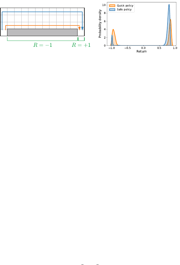
Safe policy
Quick policy
CliffsS G
Figure 2.2
Left
: The Cliffs environment, along with the path preferred by the quick and safe
policies.
Right
: The return distribution for these policies, estimated by sampling 100,000
trajectories from the environment. The figure reports the distribution as a probability
density function computed using kernel density estimation (with bandwidth 0.02).
unintended (random) direction. For simplicity, the edges of the grid act as walls.
We model falling off the cliff using a negative reward of
−
1, at which point
the episode also terminates. Reaching the tourist center yields a reward of +1
and also ends the episode. The reward is zero elsewhere. A discount factor of
γ = 0.99 incentivizes the agent to not dally too much along the way.
Figure 2.2 depicts the return distribution for two policies: a quick policy that
walks along the cliff’s edge and a safe policy that walks two cells away from
the edge.
10
The corresponding returns are bimodal, reflecting the two possible
classes of outcomes. The return distribution of the faster policy, in particular,
is sharply peaked around
−
1 and 1: the goal may be reached quickly, but the
agent is more likely to fall. 4
The next two examples show how even simple dynamics that one might
reasonably encounter in real scenarios can result in return distributions that are
markedly different from the reward distributions.
Example 2.10.
Consider a single-state, single-action Markov decision process,
so that X= {x} and A= {a}. The initial distribution is ξ
0
= δ
x
and the transition
kernel is P
X
(x | x, a) = 1. The reward has a Bernoulli distribution, with
P
R
(0 | x, a) = P
R
(1 | x, a) =
1
/2 .
Suppose we take the discount factor to be γ =
1
/2. The return is
G = R
0
+
1
2
R
1
+
1
4
R
2
+ ··· . (2.4)
10.
More precisely, the safe policy always attempts to move up when it is possible to do so, unless
it is in one of the rightmost cells. The quick policy simply moves right until one of these cells is
reached; afterward, it goes down toward the “G” cell.
Draft version.
24 Chapter 2
1.51.00.5 2.00.0
0.5
1.0
Cumulative Probability
Return
1.00.50.0
0.5
1.0
Cumulative Probability
Return
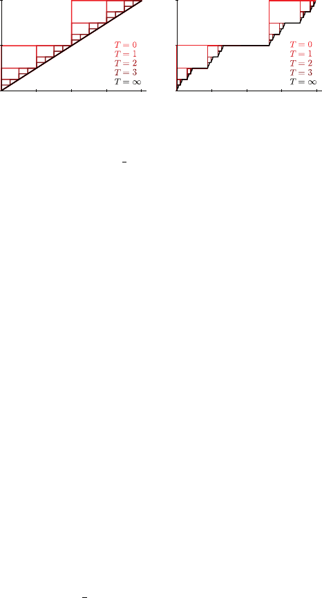
Figure 2.3
Left
: Illustration of Example 2.10, showing cumulative distribution functions (CDFs)
for the truncated return
G
0:T
=
P
T
t=0
1
2
t
R
t
as
T
increases. The number of steps in this
function doubles with each increment of
T
, reaching the uniform distribution in the limit
as T →∞. Right: The same illustration, now for Example 2.11.
We will show that
G
has a uniform probability distribution over the interval
[0
,
2]. Observe that the right-hand side of Equation 2.4 is equivalent to the
binary number
R
0
.R
1
R
2
… (2.5)
Since
R
t
∈{
0
,
1
}
for all
t
, this implies that the support of
G
is the set of numbers
that have a (possibly infinite) binary expansion as in Equation 2.5. The smallest
such number is clearly 0, while the largest number is 2 (the infinite sequence of
1s). Now
P
π
(G ∈[0, 1]) = P
π
(R
0
= 0) P
π
(G ∈[1, 2]) = P
π
(R
0
= 1) ,
so that it is equally likely that
G
falls either in the interval [0
,
1] or [1
,
2].
11
If
we now subdivide the lower interval, we find that
P
π
(G ∈[0.5, 1]) = P
π
(G ∈[0, 1])P
π
(G ≥0.5 | G ∈[0, 1])
= P
π
(R
0
= 0)P
π
(R
1
= 1 | R
0
= 0)
= P
π
(R
0
= 0)P
π
(R
1
= 1) ,
and analogously for the intervals [0
,
0
.
5]
,
[1
,
1
.
5], and [1
.
5
,
2]. We can repeat this
subdivision recursively to find that any dyadic interval [
a, b
] whose endpoints
belong to the set
Y=
n
n
X
j=0
1
2
j
a
j
: n ∈N , a
j
∈{0, 1} for 0 ≤ j ≤n
o
11. The probability that G = 1 is zero.
Draft version.

The Distribution of Returns 25
has probability
b−a
2
: that is,
P
π
G ∈[a, b]
=
b −a
2
for a, b ∈Y, a < b . (2.6)
Because the uniform distribution over the interval [0
,
2] satisfies Equation
2.6, we conclude that
G
is distributed uniformly on [0
,
2]. A formal argument
requires us to demonstrate that Equation 2.6 uniquely determines the cumulative
distribution function of
G
(Exercise 2.6); this argument is illustrated (informally)
in Figure 2.3. 4
Example 2.11
(*)
.
If we substitute the reward distribution of the previous
example by
P
R
(0 | x, a) = P
R
(
2
/3 | x, a) =
1
/2
and take
γ
=
1
/3
, the return distribution becomes the Cantor distribution (see
Exercise 2.7). The Cantor distribution has no atoms (values with probability
greater than zero) or a probability density. Its cumulative distribution function is
the Cantor function (see Figure 2.3), famous for violating many of our intuitions
about mathematical analysis. 4
2.5 The Bellman Equation
The cliff-walking scenario (Example 2.9) shows how different policies can lead
to qualitatively different return distributions: one where a positive reward for
reaching the goal is likely and one where high rewards are likely, but where
there is also a substantial chance of a low reward (due to a fall). Which should be
preferred? In reinforcement learning, the canonical way to answer this question
is to reduce return distributions to scalar values, which can be directly compared.
More precisely, we measure the quality of a policy by the expected value of its
random return,
12
or simply expected return:
E
π
h
∞
X
t=0
γ
t
R
t
i
. (2.7)
Being able to determine the expected return of a given policy is thus central
to most reinforcement learning algorithms. A straightforward approach is to
enumerate all possible realizations of the random trajectory (
X
t
, R
t
, A
t
)
t≥0
up to
length
T ∈N
. By weighting them according to their probability, we obtain the
approximation
E
π
h
T −1
X
t=0
γ
t
R
t
i
. (2.8)
12.
Our assumption that the rewards have finite first moment (Assumption 2.5) guarantees that the
expectation in Expression 2.7 is finite.
Draft version.

26 Chapter 2
However, even for reasonably small
T
, this is problematic, because the num-
ber of partial trajectories of length
T ∈N
may grow exponentially with
T
.
13
Even for problems as small as cliff-walking, enumeration quickly becomes
impractical. The solution lies in the Bellman equation, which provides a concise
characterization of the expected return under a given policy.
To begin, consider the expected return for a policy
π
from an initial state
x
.
This is called the value of x, written
V
π
(x) = E
π
∞
X
t=0
γ
t
R
t
X
0
= x
. (2.9)
The value function
V
π
describes the value at all states. As the name implies, it
is formally a mapping from a state to its expected return under policy
π
. The
value function lets us answer counterfactual questions (“how well would the
agent do from this state?”) and also allows us to determine the expected return
in Equation 2.7, since (by the generative equations)
E
π
h
V
π
(X
0
)
i
= E
π
h
∞
X
t=0
γ
t
R
t
i
.
By linearity of expectations, the expected return can be decomposed into an
immediate reward
R
0
(which depends on the initial state
X
0
) and the sum of
future rewards:
E
π
h
∞
X
t=0
γ
t
R
t
i
= E
π
h
R
0
+
∞
X
t=1
γ
t
R
t
| {z }
future rewards
i
.
The Bellman equation expresses this relationship in terms of the value of
different states; we give its proof in the next section.
Proposition 2.12
(The Bellman equation)
.
Let
V
π
be the value function
of policy π. Then for any state x ∈X, it holds that
V
π
(x) = E
π
h
R
0
+ γV
π
(X
1
) |X
0
= x
i
. (2.10)
4
The Bellman equation transforms an infinite sum (Equation 2.7) into a recur-
sive relationship between the value of a state
x
, its expected reward, and the
value of its successor states. This makes it possible to devise efficient algorithms
for determining the value function V
π
, as we shall see later.
13.
If rewards are drawn from a continuous distribution, there is in fact an infinite number of
possible sequences of length T .
Draft version.
The Distribution of Returns 27
(b)
(a)
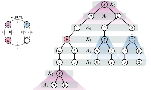
Figure 2.4
(a)
An example Markov decision process with three states
x, y, z
and a terminal state
denoted by a double circle. Action
a
gives a reward of 0 or 1 depending on the state,
while action
b
gives a reward of 0 in state
y
and 2 in state
z
. In state
x
, action
b
gives a
random reward of either 0 or 2 with equal probability. Arrows indicate the (deterministic)
transition kernel from each state.
(b)
An illustration of the Markov property (in blue):
the subsequences rooted in state
X
1
=
z
have the same probability distribution; and the
time-homogeneity property(in pink): the subsequence rooted at
X
2
=
x
has the same
probability distribution as the full sequence beginning in X
0
= x.
An alternative to the value function is the state-action value function
Q
π
. The
state-action value function describes the expected return when the action
A
0
is
fixed to a particular choice a:
Q
π
(x, a) = E
π
∞
X
t=0
γ
t
R
t
| X
0
= x, A
0
= a
.
Throughout this book, we will see a few situations for which this form is
preferred, either because it simplifies the exposition or makes certain algorithms
possible. Unless otherwise noted, the results we will present hold for both value
functions and state-action value functions.
2.6 Properties of the Random Trajectory
The Bellman equation is made possible by two fundamental properties of the
Markov decision process, time-homogeneity and the Markov property. More
precisely, these are properties of the random trajectory (
X
t
, R
t
, A
t
)
t≥0
, whose
probability distribution is described by the generative equations of Section 2.3.
To understand the distribution of the random trajectory (
X
t
, A
t
, R
t
)
t≥0
, it is
helpful to depict its possible outcomes as an infinite tree (Figure 2.4). The root
Draft version.
28 Chapter 2
of the tree is the initial state
X
0
, and each level consists of a state-action-reward
triple, drawn according to the generative equations. Each branch of the tree
then corresponds to a realization of the trajectory. Most of the quantities that
we are interested in can be extracted by “slicing” this tree in particular ways.
For example, the random return corresponds to the sum of the rewards along
each branch, discounted according to their level.
In order to relate the probability distributions of different parts of the ran-
dom trajectory, let us introduce the notation
D
(
Z
) to denote the probability
distribution of a random variable
Z
. When
Z
is real-valued we have, for
S ⊆R
,
D(Z)(S ) = P(Z ∈S ) .
One advantage of the
D
(
·
) notation is that it often avoids unnecessarily introduc-
ing (and formally characterizing) such a subset
S
and is more easily extended
to other kinds of random variables. Importantly, we write
D
π
to refer to the
distribution of random variables derived from the joint distribution
P
π
.
14
For
example,
D
π
(
R
0
+
R
1
) and
D
π
(
X
2
) are the probability distribution of the sum
R
0
+ R
1
and of the third state in the random trajectory, respectively.
The Markov property states that the trajectory from a given state
x
is inde-
pendent of the states, actions, and rewards that were encountered prior to
x
.
Graphically, this means that for a given level of the tree
k
, the identity of the
state
X
k
suffices to determine the probability distribution of the subtree rooted
at that state.
Lemma 2.13
(Markov property)
.
The trajectory (
X
t
, A
t
, R
t
)
t≥0
has the Markov
property. That is, for any k ∈N, we have
D
π
(X
t
, A
t
, R
t
)
∞
t=k
| (X
t
, A
t
, R
t
)
k−1
t=0
= (x
t
, a
t
, r
t
)
k−1
t=0
, X
k
= x
= D
π
(X
t
, A
t
, R
t
)
∞
t=k
| X
k
= x
whenever the conditional distribution of the left-hand side is defined. 4
As a concrete example, Figure 2.4 shows that there are two realizations of
the trajectory for which
X
1
=
z
. By the Markov property, the expected return
from this point on is independent of whether the immediately preceding reward
(R
0
) was 0 or 2.
One consequence of the Markov property is that the expectation of the
discounted return from time
k
is independent of the trajectory prior to time
k
,
given X
k
:
E
π
h
∞
X
t=k
γ
t
R
t
|(X
t
, A
t
, R
t
)
k−1
t=0
= (x
t
, a
t
, r
t
)
k−1
t=0
, X
k
= x
i
= E
π
h
∞
X
t=k
γ
t
R
t
|X
k
= x
i
.
14.
Because the random trajectory is infinite, the technical definition of
D
π
requires some care and
is given in Remark 2.4.
Draft version.

The Distribution of Returns 29
Time-homogeneity states that the distribution of the trajectory from a state
x
does not depend on the time
k
at which this state is visited. Graphically, this
means that for a given state
x
, the probability distribution of the subtree rooted
in that state is the same irrespective of the level k at which it occurs.
Lemma 2.14
(Time-homogeneity)
.
The trajectory (
X
t
, A
t
, R
t
)
t≥0
is time-
homogeneous, in the sense that for all k ∈N,
D
π
(X
t
, A
t
, R
t
)
∞
t=k
| X
k
= x
= D
δ
x
,π
(X
t
, A
t
, R
t
)
∞
t=0
, (2.11)
whenever the conditional distribution on the left-hand side is defined. 4
While the left-hand side of Equation 2.11 is a proper conditional distribution,
the right-hand side is derived from
P
π
(
· | X
0
=
x
) and by convention is not a
conditional distribution. With this is mind, this is why we write
D
δ
x
,π
rather
than the shorthand D
π
( · | X
0
= x).
Lemmas 2.13 and 2.14 follow as consequences of the definition of the trajec-
tory distribution. A formal proof requires some measure-theoretic treatment;
we provide a discussion of some of the considerations in Remark 2.4.
Proof of Proposition 2.12 (the Bellman equation).
The result follows straight-
forwardly from Lemmas 2.13 and 2.14. We have
V
π
(x) = E
π
h
∞
X
t=0
γ
t
R
t
| X
0
= x
i
(a)
= E
π
h
R
0
| X
0
= x
i
+ γ E
π
h
∞
X
t=1
γ
t−1
R
t
| X
0
= x
i
(b)
= E
π
h
R
0
| X
0
= x
i
+ γE
π
"
E
π
h
∞
X
t=1
γ
t−1
R
t
| X
0
= x, A
0
, X
1
i
| X
0
= x
#
(c)
= E
π
h
R
0
| X
0
= x
i
+ γE
π
"
E
π
h
∞
X
t=1
γ
t−1
R
t
| X
1
i
| X
0
= x
#
(d)
= E
π
h
R
0
| X
0
= x
i
+ γE
π
h
V
π
(X
1
) | X
0
= x
i
= E
π
R
0
+ γV
π
(X
1
) | X
0
= x
,
where (a) is due to the linearity of expectations, (b) follows by the law of
total expectation, (c) follows by the Markov property, and (d) is due to time-
homogeneity and the definition of V
π
.
The Bellman equation states that the expected value of a state can be
expressed in terms of the immediate action
A
0
, reward
R
0
, and the succes-
sor state
X
1
, omitting the rest of the trajectory. It is therefore convenient to
Draft version.
30 Chapter 2
define a generative model that only considers these three random variables along
with the initial state
X
0
. Let
ξ ∈P
(
X
) be a distribution over states. The sam-
ple transition model assigns a probability distribution to the tuple (
X, A, R, X
0
)
taking values in X×A×R ×X according to
X ∼ξ ;
A | X ∼π( · | X) ;
R |(X, A) ∼P
R
( · | X, A) ;
X
0
|(X, A, R) ∼P
X
( · | X, A) . (2.12)
We also write
P
π
for the joint distribution of these random variables. We will
often find it useful to consider a single source state
x
, such that as before
ξ
=
δ
x
. We write (
X
=
x, A, R, X
0
) for the resulting random tuple, with probability
distribution and expectation
P
π
( · | X = x) and E
π
[ · | X = x] .
The sample transition model allows us to omit time indices in the Bellman
equation, which simplifies to
V
π
(x) = E
π
R + γV
π
(X
0
) | X = x
.
In the sample transition model, we call
ξ
the state distribution. It is generally
different from the initial state distribution
ξ
0
, which describes a property of the
environment. In Chapters 3 and 6, we will use the state distribution to model
part of a learning algorithm’s behavior.
2.7 The Random-Variable Bellman Equation
The Bellman equation characterizes the expected value of the random return
from any state
x
compactly, allowing us to reduce the generative equations
(an infinite sequence) to the sample transition model. In fact, we can leverage
time-homogeneity and the Markov property to characterize all aspects of the
random return in this manner. Consider again the definition of this return as a
discounted sum of random rewards:
G =
∞
X
t=0
γ
t
R
t
.
As with value functions, we would like to relate the return from the initial state
to the random returns that occur downstream in the trajectory. To this end, let
us define the return function
G
π
(x) =
∞
X
t=0
γ
t
R
t
, X
0
= x , (2.13)
Draft version.

The Distribution of Returns 31
which describes the return obtained when acting according to
π
starting from a
given state
x
. Note that in this definition, the notation
X
0
=
x
again modifies the
initial state distribution
ξ
0
. Equation 2.13 is thus understood as “the discounted
sum of random rewards described by the generative equations with
ξ
0
=
δ
x
.”
Formally,
G
π
is a collection of random variables indexed by an initial state
x
,
each generated by a random trajectory (
X
t
, A
t
, R
t
)
t≥0
under the distribution
P
π
(
·|
X
0
=
x
). Because Equation 2.13 is concerned with random variables, we will
sometimes find it convenient to be more precise and call it the return-variable
function.
15
The infinite tree of Figure 2.4 illustrates the abstract process by which
one might generate realizations from the random variable
G
π
(
x
). We begin
at the root, whose value is fixed to
X
0
=
x
. Each level is drawn by sampling,
in succession, the action
A
t
, the reward
R
t
, and finally the successor state
X
t+1
, according to the generative equations. The return
G
π
(
x
) accumulates the
discounted rewards (γ
t
R
t
)
t≥0
along the way.
The nature of random variables poses a challenge to converting this generative
process into a recursive formulation like the Bellman equation. It is tempting to
try and formulate a distributional version of the Bellman equation by defining a
collection of random variables
˜
G
π
according to the relationship
˜
G
π
(x) = R + γ
˜
G
π
(X
0
), X = x (2.14)
for each
x ∈X
, in direct analogy with the Bellman equation for expected returns.
However, these random variables
˜
G
π
do not have the same distribution as the
random returns G
π
. The following example illustrates this point.
Example 2.15.
Consider the single-state Markov decision process of Example
2.10, for which the reward
R
has a Bernoulli distribution with parameter
1
/2
.
Equation 2.14 becomes
˜
G
π
(x) = R + γ
˜
G
π
(x) , X = x ,
which can be rearranged to give
˜
G
π
(x) =
∞
X
t=0
γ
t
R =
1
1 −γ
R .
Since R is either 0 or 1, we deduce that
˜
G
π
(x) =
0 with probability
1
/2
1
1−γ
with probability
1
/2 .
15.
One might wonder about the joint distribution of the random returns (
G
π
(
x
) :
x ∈X
). In this
book, we will (perhaps surprisingly) not need to specify this joint distribution; however, it is valid
to conceptualize these random variables as independent for concreteness.
Draft version.

32 Chapter 2
This is different from the uniform distribution identified in Example 2.10, in the
case γ =
1
/2. 4
The issue more generally with Equation 2.14 is that it effectively reuses the
reward
R
and successor state
X
0
across multiple visits to the initial state
X
=
x
,
which in general is not what we intend and violates the structure of the MDP in
question.
16
Put another way, Equation 2.14 fails because it does not correctly
handle the joint distribution of the sequence of rewards (
R
t
)
t≥0
and states (
X
t
)
t≥0
encountered along a trajectory. This phenomenon is one difference between
distributional and classical reinforcement learning; in the latter case, the issue
is avoided thanks to the linearity of expectations.
The solution is to appeal to the notion of equality in distribution. We say that
two random variables Z
1
, Z
2
are equal in distribution, denoted
Z
1
D
= Z
2
,
if their probability distributions are equal. This is effectively shorthand for
D(Z
1
) = D(Z
2
) .
Equality in distribution can be thought of as breaking up the dependency of
the two random variables on their sample spaces to compare them solely on
the basis of their probability distributions. This avoids the problem posed by
directly equating random variables.
Proposition 2.16
(
The random-variable Bellman equation
)
.
Let
G
π
be the return-variable function of policy
π
. For a sample transition
(X = x, A, R, X
0
) independent of G
π
, it holds that for any state x ∈X,
G
π
(x)
D
= R + γG
π
(X
0
), X = x . (2.15)
4
From a generative perspective, the random-variable Bellman equation states
that we can draw a sample return by sampling an immediate reward
R
and
successor state X
0
and then recursively generating a sample return from X
0
.
Proof of Proposition 2.16.
Fix
x ∈X
and let
ξ
0
=
δ
x
. Consider the (partial)
random return
G
k:∞
=
∞
X
t=k
γ
t−k
R
t
, k ∈N .
16.
Computer scientists may find it useful to view Equation 2.14 as simulating draws from
R
and
X
0
with a pseudo-random number generator that is reinitialized to the same state after each use.
Draft version.
The Distribution of Returns 33
In particular,
G
π
(
x
)
D
= G
0:∞
under the distribution
P
π
(
· | X
0
=
x
). Following an
analogous chain of reasoning as in the proof of Proposition 2.12, we decompose
the return
G
0:∞
into the immediate reward and the rewards obtained later in the
trajectory:
G
0:∞
= R
0
+ γG
1:∞
.
We can decompose this further based on the state occupied at time 1:
G
0:∞
= R
0
+ γ
X
x
0
∈X
{X
1
= x
0
}G
1:∞
.
Now, by the Markov property, on the event that
X
1
=
x
0
, the return obtained from
that point on is independent of the reward
R
0
. Further, by the time-homogeneity
property, on the same event, the return
G
1:∞
is equal in distribution to the return
obtained when the episode begins at state x
0
. Thus, we have
R
0
+ γ
X
x
0
∈X
{X
1
= x
0
}G
1:∞
D
= R
0
+ γ
X
x
0
∈X
{X
1
= x
0
}G
π
(x
0
) = R
0
+ γG
π
(X
1
) ,
and hence
G
π
(x)
D
= R
0
+ γG
π
(X
1
), X
0
= x.
The result follows by equality of distribution between (
X
0
, A
0
, R
0
, X
1
) with the
sample transition model (X = x, A, R, X
0
) when X
0
= x.
Note that Proposition 2.16 implies the standard Bellman equation, in the
sense that the latter is obtained by taking expectations on both sides of the
distributional equation:
G
π
(x)
D
= R + γG
π
(X
0
), X = x
=⇒ D
π
G
π
(x)
= D
π
R + γG
π
(X
0
) | X = x
=⇒ E
π
[G
π
(x)] = E
π
R + γG
π
(X
0
) | X = x
=⇒ V
π
(x) = E
π
R + γV
π
(X
0
) | X = x
where we made use of the linearity of expectations as well as the independence
of X
0
from the random variables (G
π
(x) : x ∈X).
2.8 From Random Variables to Probability Distributions
Random variables provide an intuitive language with which to express how
rewards are combined to form the random return. However, a proper random-
variable Bellman equation requires the notion of equality in distribution to
avoid incorrectly reusing realizations of the random reward
R
and next-state
X
0
.
Draft version.
34 Chapter 2
As a consequence, Equation 2.15 is somewhat incomplete: it characterizes the
distribution of the random return from
x
,
G
π
(
x
), but not the random variable
itself.
A natural alternative is to do away with the return-variable function
G
π
and
directly relate the distribution of the random return at different states. The result
is what we may properly call the distributional Bellman equation. Working
with probability distributions requires mathematical notation that is somewhat
unintuitive compared to the simple addition and multiplication of random
variables but is free of technical snags. With precision in mind, this is why we
call Equation 2.15 the random-variable Bellman equation.
For a real-valued random variable
Z
with probability distribution
ν ∈P
(
R
),
recall the notation
ν(S ) = P(Z ∈S ) , S ⊆R .
This allows us to consider the probability assigned to
S
by
ν
more directly,
without referring to
Z
. For each state
x ∈X
, let us denote the distribution of the
random variable G
π
(x) by η
π
(x). Using this notation, we have
η
π
(x)(S ) = P(G
π
(x) ∈S ) , S ⊆R .
We call the collection of these per-state distributions the return-distribution
function. Each
η
π
(
x
) is a member of the space
P
(
R
) of probability distributions
over the reals. Accordingly, the space of return-distribution functions is denoted
P(R)
X
.
To understand how the random-variable Bellman equation translates to the
language of probability distributions, consider that the right-hand side of Equa-
tion 2.15 involves three operations on random variables: indexing into
G
π
,
scaling, and addition. We use analogous operations over the space of probability
distributions to construct the Bellman equation for return-distribution functions;
these distributional operations are depicted in Figure 2.5.
Mixing.
Consider the return-variable and return-distribution functions
G
π
and
η
π
, respectively, as well as a source state
x ∈X
. In the random-variable
equation, the term
G
π
(
X
0
) describes the random return received at the successor
state
X
0
, when
X
=
x
and
A
is drawn from
π
(
· | X
) – hence the idea of indexing
the collection G
π
with the random variable X
0
.
Generatively, this describes the process of first sampling a state
x
0
from the
distribution of
X
0
and then sampling a realized return from
G
π
(
x
0
). If we denote
the result by G
π
(X
0
), we see that for a subset S ⊆R, we have
P
π
(G
π
(X
0
) ∈S | X = x) =
X
x
0
∈X
P
π
(X
0
= x
0
| X = x)P
π
(G
π
(X
0
) ∈S | X
0
= x
0
, X = x)
=
X
x
0
∈X
P
π
(X
0
= x
0
| X = x)P
π
G
π
(x
0
) ∈S
Draft version.
The Distribution of Returns 35
Return Return Return
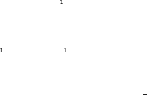
(a) (b) (c) (d)
Return
Mixing
Scaling
Translating
Figure 2.5
Illustration of the effects of the transformations of the random return in distributional
terms, for a given source state. The discount factor is applied to the individual realizations
of the return distribution, resulting in a
scaling (a)
of the support of this distribution.
The arrows illustrate that this scaling results in a “narrower” probability distribution.
The reward
r translates (b)
the return distribution. We write these two operations as a
pushforward distribution constructed from the bootstrap function
b
r,γ
. Finally, the return
distributions of successor states are combined to form a
mixture distribution (c)
whose
mixture weights are the transition probabilities to these successor states. The combined
transformations are given in
(d)
, which depicts the return distribution at the source state
(dark outline).
=
X
x
0
∈X
P
π
(X
0
= x
0
| X = x)η
π
(x
0
)
(S ) . (2.16)
This shows that the probability distribution of
G
π
(
X
0
) is a weighted combination,
or mixture of probability distributions from η
π
. More compactly, we have
D
π
G
π
(X
0
) | X = x
=
X
x
0
∈X
P
π
(X
0
= x
0
| X = x)η
π
(x
0
)
= E
π
η
π
(X
0
) | X = x
.
Consequently, the distributional analogue of indexing into the collection
G
π
of
random returns is the mixing of their probability distributions.
Although we prefer working directly with probability distributions, the
indexing step also has a simple expression in terms of cumulative distribu-
tion functions. In Equation 2.16, taking the set
S
to be the half-open interval
(−∞, z], we obtain
P
π
(G
π
(X
0
) ≤z | X = x) = P
π
(G
π
(X
0
) ∈(−∞, z] | X = x)
=
X
x
0
∈X
P
π
(X
0
= x
0
| X = x)P
π
(G
π
(x
0
) ≤z) .
Thus, the mixture of next-state return distributions can be described by the
mixture of their cumulative distribution functions:
F
G
π
(X
0
)
(z) =
X
x
0
∈X
P
π
(X
0
= x
0
| X = x)F
G
π
(x
0
)
(z) .
Draft version.

36 Chapter 2
Scaling and translation.
Suppose we are given the distribution of the next-
state return
G
π
(
X
0
). What is then the distribution of
R
+
γG
π
(
X
0
)? To answer this
question, we must express how multiplying by the discount factor and adding a
fixed reward r transforms the distribution of G
π
(X
0
).
This is an instance of a more general question: given a random variable
Z ∼ν
and a transformation
f
:
R →R
, how should we express the distribution
of
f
(
Z
) in terms of
f
and
ν
? Our approach is to use the notion of a pushforward
distribution. The pushforward distribution
f
#
ν
is defined as the distribution of
f (Z):
f
#
ν = D
f (Z)
.
One can think of it as applying the function
f
to the individual realizations of this
distribution – “pushing” the mass of the distribution around. The pushforward
notation allows us to reason about the effects of these transformations on
distributions themselves, without having to involve random variables.
Now, for two scalars
r ∈R
and
γ ∈
[0
,
1), let us define the bootstrap function
b
r,γ
: z 7→r + γz .
The pushforward operation applied with the bootstrap function scales each
realization by γ and then adds r to it. That is,
(b
r,γ
)
#
ν = D(r + γZ) . (2.17)
Expressed in terms of cumulative distribution functions, this is
F
r+γZ
(z) = F
Z
z −r
γ
.
We use the pushforward operation and the bootstrap function to describe
the transformation of the next-state return distribution by the reward and the
discount factor. If x
0
is a state with return distribution η
π
(x
0
), then
(b
r,γ
)
#
η
π
(x
0
) = D
r + γG
π
(x
0
)
.
We finally combine the pushforward and mixing operations to produce a
probability distribution
b
r,γ
#
E
π
η
π
(X
0
) | X = x
= E
π
h
b
r,γ
#
η
π
(X
0
) | X = x
i
, (2.18)
by linearity of the pushforward (see Exercises 2.11–2.13).
Equation 2.18 gives the distribution of the random return for a specific
realization of the random reward
R
. By taking the expectation over
R
and
X
0
,
we obtain the distributional Bellman equation.
Draft version.

The Distribution of Returns 37
Proposition 2.17
(
The distributional Bellman equation
)
.
Let
η
π
be the
return-distribution function of policy π. For any state x ∈X, we have
η
π
(x) = E
π
[(b
R,γ
)
#
η
π
(X
0
) |X = x] . (2.19)
4
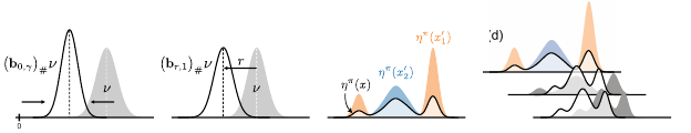
Figure 2.6 illustrates the recursive relationship between return distributions
described by the distributional Bellman equation.
Example 2.18.
In Example 2.10, it was determined that the random return at
state
x
is uniformly distributed on the interval [0
,
2]. Recall that there are two
possible rewards (0 and 1) with equal probability,
x
transitions back to itself,
and γ =
1
/2. As X
0
= x, when r = 0, we have
E
π
h
b
r,γ
#
η
π
(X
0
) | X = x
i
= (b
0,γ
)
#
η
π
(x)
= D
γG
π
(x)
= U([0, 2γ])
= U([0, 1]) .
Similarly, when r = 1, we have
(b
1,γ
)
#
η
π
(x) = D
1 + γG
π
(x)
= U([1, 2]) .
Consequently,
D
π
R + γG
π
(X
0
) | X = x
=
1
2
(b
0,γ
)
#
η
π
(x) +
1
2
(b
1,γ
)
#
η
π
(x)
=
1
2
U([0, 1]) +
1
2
U([1, 2])
= U([0, 2])
= η
π
(x) .
This illustrates how the pushforward operation can be used to express, in
distributional terms, the transformations at the heart of the random-variable
Bellman equation. 4
Proposition 2.17 can also be stated in terms of cumulative distribution func-
tions. Halfway between Equation 2.19 and the random-variable equation, what
one might call the cumulative distribution function Bellman equation is
F
G
π
(x)
(z) = E
π
F
R+γG
π
(X
0
)
(z) | X = x
Draft version.

38 Chapter 2
= E
π
h
F
G
π
(X
0
)
z −R
γ
| X = x
i
.
The first form highlights the relationship between the random-variable equation
and the distributional equation, whereas the second form more directly expresses
the relationship between the different cumulative distribution functions; the
odd indexing reflects the process of transferring probability mass “backward,”
from
G
π
(
X
0
) to
G
π
(
x
). Although the cumulative distribution function Bellman
equation is at first glance simpler than Equation 2.19, in later chapters, we
will see that working with probability distributions is usually more natural and
direct.
Proof of Proposition 2.17.
Let
S ⊆R
and fix
x ∈X
. By the law of total
expectation, we may write
P
π
(R + γG
π
(X
0
) ∈S | X = x)
=
X
a∈A
π(a | x)
X
x
0
∈X
P
X
(x
0
| x, a)P
π
R + γG
π
(X
0
) ∈S | X = x, A = a, X
0
= x
0
)
(a)
=
X
a∈A
π(a | x)
X
x
0
∈X
P
X
(x
0
| x, a) ×
E
R
h
P
π
R + γG
π
(x
0
) ∈S | X = x, A = a, R
| X = x, A = a
i
=
X
a∈A
π(a | x)
X
x
0
∈X
P
X
(x
0
| x, a) E
R
h
(b
R,γ
)
#
η
π
(x
0
)
(S ) | X = x, A = a
i
= E
π
h
(b
R,γ
)
#
η
π
(X
0
)
(S ) | X = x
i
= E
π
(b
R,γ
)
#
η
π
(X
0
) | X = x
i
(S ) .
The notation
E
R
in (
a
) denotes the expectation with respect to
R ∼P
R
(
· | x, a
);
the independence of
R
and
X
0
given
A
allows us to remove the conditional
X
0
=
x
0
from the inner probability term. Now, by Proposition 2.16, we know that
G
π
(x)
D
= R + γG
π
(X
0
), X = x .
By definition,
η
π
(
x
) is the distribution of
G
π
(
x
) and hence the distribution of
R
+
γG
π
(
X
0
) when
X
=
x
. But the derivation above shows that that distribution
is
E
π
(b
R,γ
)
#
η
π
(X
0
) | X = x
,
which completes the proof.
Equation 2.19 directly relates the return distributions at different states and
does away with the return-variable function
G
π
. This makes it particularly useful
when mathematical rigor is required, such as to prove the more formal results
Draft version.
The Distribution of Returns 39
Return
Return
Return
Reward
Reward
Reward
Reward
Reward
Reward
Return
Figure 2.6
The distributional Bellman equation states that the return distribution at one state (far
left) is formed by scaling the return distributions at successor states, shifting them by the
realized rewards, and mixing over possible realizations.
in later chapters. The random variables
X
,
R
, and
X
0
remain, however, inside
the expectation on the right-hand side. Their role is to concisely express the
three operations of mixing, scaling, and translation. It is also possible to omit
these random variables and write Equation 2.19 purely in terms of probability
distributions, by making the expectation explicit:
η
π
(x) =
X
a∈A
π(a | x)
X
x
0
∈X
P
X
(x
0
| x, a)
Z
R
P
R
(dr | x, a)
b
r,γ
)
#
η
π
(x
0
) , (2.20)
as was partially done in the proof above. We will revisit this form of the
distributional Bellman equation in Chapter 5 when we consider algorithms for
approximating the return distribution. In general, however, Equation 2.19 is
more compact and applies equally well to discrete and continuous distributions.
Observe that the random action
A
is implicit in the random-variable and
distributional Bellman equations but explicit in Equation 2.20. This is because
A
is needed to determine the probability distributions of
R
and
X
0
, which are
only independent conditional on the action. This is a useful reminder that we
need to treat the addition of
R
to
γG
π
(
X
0
) with care – these are not in general
independent random variables, and their addition does not generally correspond
to a simple convolution of distributions. We will consider this issue in more
detail in Chapter 4.
Draft version.

40 Chapter 2
2.9 Alternative Notions of the Return Distribution*
In reinforcement learning, the discount factor
γ
is typically presented as a scalar
multiplier that shrinks the magnitude of future rewards. This is the interpretation
we have used to present the return in this chapter. However, the discount factor
can be given a different interpretation as a probability of continuing. Under this
alternate interpretation, the rewards received by the agent are undiscounted, and
instead there is a probability 1
−γ
that the sequence terminates at each time
step.
Under this model, the agent’s interactions with its environment end after a
random termination time
T
, which is geometrically distributed with parameter
γ
, independently of all other random variables in the sequence. Specifically,
we have
P
π
(
T
=
t
) =
γ
t
(1
−γ
) for all
t ≥
0. In this case, the agent’s return is now
given by
T
X
t=0
R
t
.
We call this the random-horizon return.
Straightforward calculation allows us to show that the expected value of the
return is unchanged (see Exercise 2.14):
E
π
T
X
t=0
R
t
= E
π
∞
X
t=0
γ
t
R
t
.
Because of this equivalence, from an expected-return perspective, it does not
matter whether
γ
is interpreted as a scaling factor or probability. By contrast,
this change in interpretation of
γ
has a significant impact on the structure of
the return distribution. For example, the random variable
P
T
t=0
R
t
is unbounded
even when the rewards are bounded, unlike the discounted return.
Just as there exists a distributional Bellman equation for the discounted return,
there is also a recursive characterization of the return distribution for this variant
of the return. By introducing an auxiliary random variable
I
=
{T > 0}
, we can
write down a distributional Bellman equation for this alternative interpretation
of the return. Expressing this relationship in terms of random variables, we have
G
π
(x)
D
= R + IG
π
(X
0
), X = x .
In terms of distributions themselves, we have
η
π
(x) = (1 −γ)D
π
(R | X = x) + γE
π
(b
R,1
)
#
η
π
(X
0
) |X = x
,
where
D
π
(
R | X
=
x
) denotes the distribution of the reward
R
at
x
under
π
.
Notice that
γ
in the equation above, which previously scaled the support of the
distribution, now mixes two probability distributions. These results are proven
Draft version.
The Distribution of Returns 41
in the course of Exercise 2.15 along with similar results for a more general class
of return definitions. The fact that there exists a distributional Bellman equation
for these variants of the return means that much of the theory of distributional
reinforcement learning still applies. We encourage the reader to consider how
the algorithms and analysis presented in later chapters may be modified to
accommodate alternative notions of the return.
We see that there are multiple ways in which we can define distributional
Bellman equations while preserving the relationship between expectations.
Another approach, commonly known as
n
-step bootstrapping in reinforcement
learning, relates the return distribution at state
x
with the return distribution
n
steps into the future. Exercise 2.16 describes another alternative based on first
return times.
2.10 Technical Remarks
Remark 2.1.
Our account of random variables in this chapter has not required
a measure-theoretic formalism, and in general this will be the case for the
remainder of the book. For readers with a background in measure theory, the
existence of the joint distribution of the random variables (
X
t
, A
t
, R
t
)
t≥0
in the
Markov decision process model described in this chapter can be deduced from
constructing a consistent sequence of distributions for the random variables
(
X
t
, A
t
, R
t
)
H
t=0
for each horizon
H ∈N
using the conditional distributions given in
the definition and then appealing to the Ionescu Tulcea theorem (Tulcea 1949).
See Lattimore and Szepesvári (2020) for further discussion in the context of
Markov decision processes.
We also remark that a more formal definition of probability measures restricts
the subsets of outcomes under consideration to be measurable with an under-
lying
σ
-algebra. Here, and elsewhere in the book, we will generally avoid
repeated mention of the qualifier “measurable” in cases such as these. The issue
can be safely ignored by readers without a background in measure theory. For
readers with such a background, measurability is always implicitly with respect
to the power set
σ
-algebra on finite sets, the Borel
σ
-algebra on the reals, and
the corresponding product σ-algebra on products of such spaces. 4
Remark 2.2.
The existence of the random return
P
∞
t=0
γ
t
R
t
is often taken for
granted in reinforcement learning. In part, this is because assuming that rewards
are deterministic or have distributions with bounded support makes its existence
straightforward; see Exercise 2.17.
The situation is more complicated when the support of the reward distribu-
tions is unbounded, as there might be realizations of the random trajectory for
which the sequence (
G
0:T
)
T ≥0
does not converge. If, for example, the rewards
Draft version.
42 Chapter 2
are normally distributed, then it is possible that
R
0
= 1
, R
1
=
−γ
−1
, R
2
=
γ
−2
, R
3
=
−γ
−3
, . . .
, in which case
G
0:T
oscillates between 0 and 1 indefinitely. When the
truncated returns do not converge, it is not meaningful to talk about the return
obtained in this realization of the trajectory.
Under the assumption that all reward distributions have finite mean, we can
demonstrate convergence of the truncated return with probability 1:
P
lim
T →∞
T
X
t=0
γ
t
R
t
exists
= 1 , (2.21)
and hence guarantee that we can meaningfully study the distributional properties
of the random return. Intuitively, problematic sequences of rewards such as the
sequence given above require reward samples that are increasingly “unlikely”.
Equation 2.21 is established by appealing to the martingale convergence
theorem, and the details of this derivation are explored in Exercise 2.19. 4
Remark 2.3.
The assumption of finite state and action spaces makes several
technical aspects of the presentation in this book more straightforward. As a
simple example, consider a Markov decision process with countably infinite
state space given by the nonnegative integers
N
, for which state
x
deterministi-
cally transitions to state
x
+ 1. Suppose in addition that the trajectory begins in
state 0. If the reward at state
x
is (
−γ
)
−x
, then the truncated return up to time
T
is given by
T −1
X
t=0
γ
t
R
t
=
T −1
X
t=0
γ
t
(−γ)
−t
=
T −1
X
t=0
(−1)
−t
.
In the spirit of Remark 2.2, when
T
is odd, this sum is 1, while for
T
even, it
is 0. Hence, the limit
P
∞
t=0
γ
t
R
t
does not exist, despite the fact that all reward
distributions have finite mean.
Dealing with continuous state spaces requires more technical sophistication
still. Constructing the random variables describing the trajectory requires taking
into account the topology of the state space in question, and careful consider-
ation of technical conditions on policies (such as measurability) is necessary
too. For details on how these issues may be addressed, see Puterman (2014)
and Meyn and Tweedie (2012). 4
Remark 2.4
(Proof of time-homogeneity and the Markov property)
.
The gener-
ative equations defining the distribution of the random trajectory (
X
t
, A
t
, R
t
)
t≥0
immediately give statements such as
P
π
(X
k+1
= x
0
| X
0:k
, A
0:k
, R
0:k
, X
k
) = P
π
(X
k+1
= x
0
| X
k
) ,
Draft version.
The Distribution of Returns 43
which shows that the next state in the trajectory enjoys the Markov property.
Lemmas 2.13 and 2.14 state something stronger: that the entire future trajectory
has this property. To prove these lemmas from the generative equations, the strat-
egy is to note that the distribution of (
X
t
, A
t
, R
t
)
∞
t=k
conditional on (
X
t
, A
t
, R
t
)
k−1
t=0
and
X
k
is determined by its finite-dimensional marginal distributions: that is,
conditional probabilities of the form
P
π
(X
t
i
= x
i
, A
t
i
= a
i
, R
t
i
∈S
i
for i = 1, …, n | (X
t
, A
t
, R
t
)
k−1
t=0
, X
k
)
for all
n ∈N
+
and sequences
k ≤t
1
< ···< t
n
of time steps (see, e.g., Billingsley
2012, Section 36). Thus, if these conditional probabilities are equal to the
corresponding quantities
P
π
(X
t
i
= x
i
, A
t
i
= a
i
, R
t
i
∈S
i
for i = 1, …, n | X
k
) ,
then the distributions are equal. Finally, the equality of these finite-dimensional
marginals can be shown by induction from the generative equations. 4
2.11 Bibliographical Remarks
An introduction to random variables and probability distributions may be found
in any undergraduate textbook on the subject. For a more technical presentation,
see Williams (1991) and Billingsley (2012).
2.2.
Markov decision processes are generally attributed to Bellman (1957b). A
deeper treatment than we give here can be found in most introductory textbooks,
including those by Bertsekas and Tsitsiklis (1996), Szepesvári (2010), and
Puterman (2014). Our notation is most aligned with that of Sutton and Barto
(2018). Interestingly, while it is by now standard to use reward as an indicator
of success, Bellman’s own treatment does not make it an integral part of the
formalism.
2.3.
The formulation of a trajectory as a sequence of random variables is central
to control as inference (Toussaint 2009; Levine 2018), which uses tools from
probabilistic reasoning to derive optimal policies. Howard (1960) used the
analogy of a frog hopping around a lily pond to convey the dynamics of a
Markov decision process; we find our own analogy more vivid. The special
consideration owed to infinite sequences is studied at length by Hutter (2005).
2.4.
The work of Veness et al. (2015) makes the return (as a random variable)
the central object of interest and is the starting point of our own investigations
into distributional reinforcement learning. Issues regarding the existence of
the random return and a proper probabilistic formulation can be found in that
paper. An early formulation of the return-variable function can be found in
Jaquette (1973), who used it to study alternative optimality criteria. Chapman
and Kaelbling (1991) consider the related problem of predicting the discounted
Draft version.
44 Chapter 2
cumulative probability of observing a particular level of reward in order to
mitigate partial observability in a simple video game. The blackjack and cliff-
walking examples are adapted from Sutton and Barto (2018) and, in the latter
case, inspired by one of the authors’ trip to Ireland. In both cases, we put
a special emphasis on the probability distribution of the random return. The
uniform distribution example is taken from Bellemare et al. (2017a); such
discounted sums of Bernoulli random variables also have a long history in
probability theory (Jessen and Wintner 1935; see Solomyak 1995; Diaconis and
Freedman 1999; Peres et al. 2000 and references therein).
2.5–2.6.
The Bellman equation is standard to most textbooks on the topic. A
particularly thorough treatment can be found in the work of Puterman (2014)
and Bertsekas (2012). The former also provides a good discussion on the
implications of the Markov property and time-homogeneity.
2.7–2.8.
Bellman equations relating quantities other than expected returns were
originally introduced in the context of risk-sensitive control, at varying levels
of generality. The formulation of the distributional Bellman equation in terms
of cumulative distribution functions was first given by Sobel (1982), under the
assumption of deterministic rewards and policies. Chung and Sobel (1987) later
gave a version for random, bounded rewards. See also the work of White (1988)
for a review of some of these approaches and Morimura et al. (2010a) for a
more recent presentation of the CDF Bellman equation.
Other versions of the distributional Bellman equation have been phrased in
terms of moments (Sobel 1982), characteristic functions (Mandl 1971; Farah-
mand 2019), and the Laplace transform (Howard and Matheson 1972; Jaquette
1973, 1976; Denardo and Rothblum 1979), again at varying levels of general-
ity, and in some cases using the undiscounted return. Morimura et al. (2010b)
also present a version of the equation in terms of probability densities. The
formulation of the distributional Bellman equation in terms of pushforward dis-
tributions is due to Rowland et al. (2018); the pushforward notation is broadly
used in measure-theoretic probability, and our use of it is influenced by optimal
transport theory (Villani 2008).
Distributional formulations have also been used to design Bayesian methods
for reasoning about uncertainty regarding the value function (Ghavamzadeh et
al. 2015). Dearden et al. (1998) propose an algorithm that maintains a posterior
on the return distribution under the assumption that rewards are normally
distributed. Engel et al. (2003, 2007) use a random-variable equation to derive
an algorithm based on Gaussian processes.
Our own work in the field is rooted in the theory of stochastic fixed point
equations (Rösler 1991, 1992; Rachev and Rüschendorf 1995), also known as
recursive distributional equations (Aldous and Bandyopadhyay 2005), from
Draft version.
The Distribution of Returns 45
which we draw the notion of equality in distribution. Recursive distributional
equations have been used, among other applications, for complexity analysis of
randomized algorithms (Rösler and Rüschendorf 2001), as well as the study of
branching processes and objects in random geometry (Liu 1998). See Alsmeyer
(2012) for a book-length survey of the field. In effect, the random-variable
Bellman equation for a given state
x
is a recursive distributional equation in the
sense of Aldous and Bandyopadhyay (2005); however, in distributional rein-
forcement learning, we typically emphasize the collection of random variables
(the return-variable function) over individual equations.
2.9.
The idea of treating the discount factor as a probability recurs in the
literature, often as a technical device within a proof. Our earliest source is
Derman (1970, Chap. 3). The idea is used to handle discounted, infinite horizon
problems in the reinforcement learning as inference setting (Toussaint and
Storkey 2006) and is remarked on by Sutton et al. (2011). The probabilistic
interpretation of the discount factor has also found application in model-based
reinforcement learning (Sutton 1995; Janner et al. 2020), and is closely related
to the notion of termination probabilities in options (Sutton et al. 1999). The
extension to the distributional setting was worked out with Tom Schaul but
not previously published. See also White (2017) for a broader discussion on
unifying various uses of discount factors.
2.12 Exercises
Exercise 2.1. We defined a state x as being terminal if
P
X
(x | x, a) = 1 for all a ∈A
and P
R
(0 | x, a) = 1.
(i)
Explain why multiple terminal states are redundant from a return function
perspective.
(ii)
Suppose you are given an MDP with
k
terminal states. Describe a procedure
that creates a new MDP that behaves identically but has a single terminal
state. 4
Exercise 2.2.
Consider the generative equations of Section 2.3. Using Bayes’s
rule, explain why
P
π
(X
1
= x
0
| X
0
= x, A
0
= a)
needs to be introduced as a notational convention, rather than derived from the
definition of the joint distribution P
π
. 4
Draft version.

46 Chapter 2
Exercise 2.3. Suppose that γ < 1 and R
t
∈[R
min
, R
max
] for all t ∈N. Show that
∞
X
t=0
γ
t
R
t
∈
"
R
min
1 −γ
,
R
max
1 −γ
#
. 4
Exercise 2.4.
Find a probability distribution
ν
that has unbounded support and
such that
P
π
∞
X
t=0
γ
t
Z
t
< ∞
= 1 , Z
t
i.i.d.
∼ ν for t ∈N . 4
Exercise 2.5. Using an open-source implementation of the game of blackjack
or your own, use simulations to estimate the probability distribution of the
random return under
(i) The uniformly random policy.
(ii)
The policy that doubles when starting with 10 or 11, hits on 16 and lower,
and otherwise sticks.
(iii)
The policy that hits on 16 and lower and never doubles. Is it a better
policy? 4
In all cases, aces should count as 11 whenever possible.
Exercise 2.6.
Show that any random variable
Z
satisfying the condition in
Equation 2.6 must have CDF given by
P
π
Z ≤z
=
z
2
, 0 ≤z ≤2 ,
and hence that Z has distribution U([0, 2]). 4
Exercise 2.7
(*)
.
The Cantor distribution has a cumulative distribution function
F, defined for z ∈[0, 1] by expressing z in base 3:
z =
∞
X
n=1
z
n
3
−n
, z
n
∈{0, 1, 2},
such that
F(z) =
∞
X
n=1
{z
n
> 0 , z
i
, 1 for all 1 ≤i < n}2
−n
.
Additionally,
F
(
z
) = 0 for
z ≤
0 and
F
(
z
) = 1 for
z ≥
1. Prove that the return
distribution for the MDP in Example 2.11 is the Cantor distribution. 4
Exercise 2.8.
The
n
-step Bellman equation relates the value function at a state
x
with the discounted sum of
n ∈N
+
future rewards and the value of the
n
th
successor state. Prove that, for each n ∈N
+
,
V
π
(x) = E
π
h
n−1
X
t=0
γ
t
R
t
+ γ
n
V
π
(X
n
) | X
0
= x
i
. 4
Draft version.
The Distribution of Returns 47
Exercise 2.9.
In Section 2.5, we argued that the number of partial trajectories
of length
T
can grow exponentially with
T
. Give examples of Markov decision
processes with
N
X
states and
N
A
actions where the number of possible length
T realizations (x
t
, a
t
, r
t
)
T
t=0
of the random trajectory is
(i) Bounded by a constant.
(ii) Linear in T . 4
Exercise 2.10. In Section 2.7, we argued that the equation
˜
G
π
(x) = R + γ
˜
G
π
(X
0
) , X = x
leads to the wrong probability distribution over returns. Are there scenarios in
which this is a sensible model? 4
Exercise 2.11.
The purpose of this exercise is to familiarize yourself with the
transformations of the pushforward operation applied to the bootstrap function
b
. Let
ν ∈P
(
R
) be a probability distribution and let
Z
be a random variable
with distribution
ν
. Let
r
=
1
/2
,
γ
=
1
/3
, and let
R
be a Bernoulli(
1
/4
) random
variable independent of Z. For each of the following probability distributions:
(i) ν = δ
1
;
(ii) ν =
1
/2δ
−1
+
1
/2δ
1
;
(iii) ν = N(2, 1),
express the probability distributions produced by the following operations:
(i) (b
r,1
)
#
ν = D(r + Z);
(ii) (b
0,γ
)
#
ν = D(γZ);
(iii) (b
r,γ
)
#
ν = D(r + γZ); and
(iv) E[(b
R,γ
)
#
ν] = D(R + γZ) . 4
Exercise 2.12.
Repeat the preceding exercise, now with
R ∼N
(0
,
1). Conclude
on the distribution of the random return
G =
∞
X
t=0
γ
t
R
t
,
where R
t
∼N(1, 1) for all t ≥0. 4
Exercise 2.13.
Let
η ∈P
(
R
)
X
be a return-distribution function, and let
X
0
be a
X
-valued random variable. Show that for any
r, γ ∈R
, the pushforward
operation combined with the bootstrap function forms an affine map, in the
sense that
b
r,γ
#
E
η(X
0
)
= E
b
r,γ
#
η(X
0
)
. 4
Draft version.

48 Chapter 2
Exercise 2.14.
Consider the standard discounted return
P
∞
t=0
γ
t
R
t
. Recall from
Section 2.9 the random-horizon return,
P
T
t=0
R
t
, where
T
has a geometric
probability distribution with parameter γ:
P
π
(T = k) = γ
k
(1 −γ) .
Show that
E
π
∞
X
t=0
γ
t
R
t
= E
π
T
X
t=0
R
t
. 4
Exercise 2.15.
Consider again the random-horizon return described in
Section 2.9.
(i)
Show that if the termination time
T
has a geometric distribution with
parameter
γ
, then
T
has the memoryless property: that is,
P
π
(
T ≥k
+
l |T ≥
k) = P
π
(T ≥l), for all k, l ∈N.
(ii)
Hence, show that the return-variable function corresponding to this
alternative definition of return satisfies the Bellman equation
G
π
(x)
D
= R +
{T > 0}
G
π
(X
0
), X = x .
for each x ∈X.
Consider now a further alternative notion of return, given by considering a
sequence of identically and independent distributed (i.i.d.) nonnegative random
variables (
I
t
)
t≥0
, independent from all other random variables in the MDP.
Suppose E
π
[I
t
] = γ. Define the return to be
∞
X
t=0
t−1
Y
s=0
I
s
R
t
.
(iii)
Show that both the standard definition of the return and the random-horizon
return can be viewed as special cases of this more general notion of return
by particular choices of the distribution of the (I
t
)
t≥0
variables.
(iv) Verify that
E
π
h
∞
X
t=0
t−1
Y
s=0
I
s
R
t
i
= E
π
h
∞
X
t=0
γ
t
R
t
i
.
(v)
Show that the random-variable Bellman equation associated with this
notion of return is given by
G
π
(x) = R + I
0
G
π
(X
0
) , X = x
for each x ∈X. 4
Exercise 2.16. For a state x ∈X, write
T
x
= min{t ≥1 : X
t
= x}
Draft version.

The Distribution of Returns 49
with
T
x
=
∞
if
x
is never reached from time
t
= 1 onward. When
X
0
=
x
, this
is the random time of first return to
x
. Prove that the following alternative
random-variable Bellman equation holds:
G
π
(x)
D
=
T −1
X
t=0
γ
t
R
t
+ γ
T
G
π
(x), X
0
= x . 4
Exercise 2.17.
The aim of the following two exercises is to explore under what
conditions the random return
G
=
P
∞
t=0
γ
t
R
t
exists. As in Remark 2.2, denote
the truncated return by
G
0:T
=
T
X
t=0
γ
t
R
t
.
Show that if all reward distributions are supported on the interval [
R
min
, R
max
],
then for any values of the random variables (
R
t
)
t≥0
, the sequence (
G
0:T
)
T ≥0
converges, and hence G is well defined. 4
Exercise 2.18 (*). The random-variable Bellman equation is effectively a sys-
tem of recursive distributional equations (Aldous and Bandyopadhyay 2005).
This example asks you to characterize the normal distribution as the solution to
another such equation. Let
Z
be a normally distributed random variable with
mean zero and unit variance (that is,
Z ∼N
(0
,
1)). Recall that the probability
density p
Z
and characteristic function χ
Z
of Z are
p
Z
(z) =
1
√
2π
exp
−
z
2
2
, χ
Z
(s) = exp
−
s
2
2
.
Suppose that Z
0
is an independent copy of Z. Show that
Z
D
= 2
−
1
/2
Z + 2
−
1
/2
Z
0
by considering
(i) the probability density of each side of the equation above;
(ii) the characteristic function of each side of the equation above. 4
Exercise 2.19
(*)
.
Under the overarching assumption of this chapter and
the remainder of the book that there are finitely many states and all reward
distributions have finite first moment, we can show that the limit
lim
T →∞
T
X
t=0
γ
t
R
t
(2.22)
exists with probability 1. First, show that the sequence of truncated returns
(
G
0:T
)
T ≥0
forms a semi-martingale with respect to the filtration (
F
t
)
t≥0
, defined
by
F
t
= σ(X
0:t
, A
0:t
, R
0:t−1
) ;
Draft version.
50 Chapter 2
the relevant decomposition is
G
0:T
= G
0:T −1
+ γ
t
E
π
[R
T
| X
T
, A
T
]
| {z }
predictable increment
+ γ
t
(R
T
−E
π
[R
T
| X
T
, A
T
])
| {z }
martingale noise
.
Writing
C
T
=
T
X
t=0
γ
t
E
π
[R
t
| X
t
, A
t
]
for the sum of predictable increments, show that this sequence converges for
all realizations of the random trajectory. Next, show that the sequence (
¯
C
T
)
T ≥0
defined by
¯
C
T
=
G
0:T
−C
T
is a martingale, and by using the assumption of a
finite state space X, show that it satisfies
sup
T ≥0
E[|
¯
C
T
|] < ∞.
Hence, use the martingale convergence theorem to argue that (
¯
C
T
)
T ≥0
converges
with probability 1 (w.p. 1). From there, deduce that the limit of Equation 2.22
exists w.p. 1. 4
Exercise 2.20
(*)
.
The second Borel–Cantelli lemma (Billingsley 2012,
Section 4) states that if (
E
t
)
t≥0
is a sequence of independent events and
P
t≥0
P(E
t
) = ∞, then
P(infinitely many E
t
occur) = 1 .
Let
ε >
0. Exhibit a Markov decision process and policy for which the events
{|γ
t
R
t
|> ε} are independent, and satisfy
P
π
(|γ
t
R
t
|> ε for infinitely many t) = 1 .
Deduce that
P
π
T
X
t=0
γ
t
R
t
converges as T →∞
= 0
in this case. Hint. Construct a sufficiently heavy-tailed reward distribution from
a suitable cumulative distribution function. 4
Draft version.