11
Two Applications and a Conclusion
We conclude by highlighting two applications of the core ideas covered in
earlier chapters, with the aim to give a sense of the range of domains to which
ideas from distributional reinforcement learning have been and may eventually
be applied.
11.1 Multiagent Reinforcement Learning
The core setting studied in this book is the interaction between an agent and its
environment. The model of the environment as an unchanging, static Markov
decision process is a good fit for many problems of interest. However, a notable
exception is the case in which the agent finds itself interacting with other
learning agents. Such settings arise in games, both competitive and cooperative,
as well as real-world interactions such as in autonomous driving.
Interactions between distinct agents lead to an incredibly rich space of learn-
ing problems. What is possible is governed by considerations such as how
many agents there are, whether their interests are aligned or competing, whether
they have the same information about the environment, whether they must act
concurrently or sequentially, and whether they can directly communicate with
each other. We choose to focus here on just one of many models for cooperative
multiagent interactions.
Definition 11.1
(Boutilier 1996)
.
A multiagent Markov decision process
(MMDP) is a Markov decision process (
X, A, ξ
0
, P
X
, P
R
) in which the action
set
A
has a factorized structure
A
=
Q
N
i=1
A
i
, for some integer
N ∈N
+
and finite
nonempty sets A
i
. We refer to N as the number of players in the MMDP. 4
An
N
-player MMDP describes
N
agents interacting with an environment. At
each stage, agent
i
selects an action
a
i
∈A
i
(
i
= 1
, …, N
), knowing the current
state
x ∈X
of the MMDP, but without knowledge of the actions of the other
agents. All agents observe the reward resulting from the joint action (
a
1
, …, a
N
)
Draft version. 319
320 Chapter 11
and share the joint goal of maximizing the discounted sum of rewards arising in
the MMDP; their interests are perfectly aligned.
To compute a joint optimal policy for the agents, one approach is to treat
the problem as an MDP and use either dynamic programming or temporal-
difference learning methods to compute an optimal policy. These methods
assume centralized computation of the policy, which is then communicated to
the agents to execute.
By contrast, the decentralized control problem is for the agents to arrive
at a joint optimal policy through direct interaction with the environment and
without any centralized or interagent communication; this is pertinent when
communication between agents is impossible or costly, and a model of the
environment is not known. Thus, the agents jointly interact with the environment,
producing transitions of the form (
x,
(
a
1
, …, a
N
)
, r, x
0
); agent
i
observes only
(
x, a
i
, r, x
0
) and must learn from transitions of this form, without observing the
actions of other agents that influenced the transition.
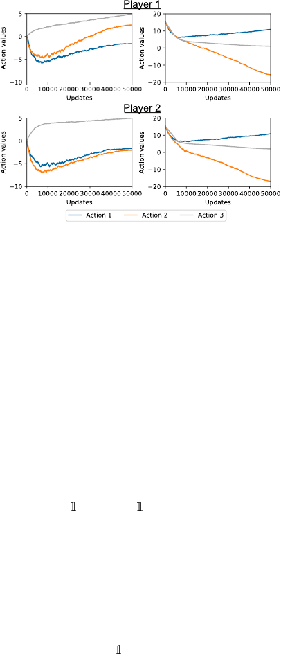
Example 11.2.
The partially stochastic climbing game (Kapetanakis and
Kudenko 2002; Claus and Boutilier 1998) is an MMDP with a single non-
terminal state (also known as a matrix game), two players, and three actions per
player. The reward distributions for each combination of the players’ actions
are shown on the left-hand side of Figure 11.1; the first player’s actions index
the rows of this matrix, and the second player’s actions index the columns. All
rewards are deterministic, except for the case of the central element, where
the distribution is uniform over the set
{
0
,
14
}
. This environment represents a
coordination challenge for the two agents: the optimal strategy is for both to
take the first action, but if either agent deviates from this strategy (by exploring
the value of other actions, for example), negative rewards of large magnitude
are incurred. 4
A concrete example of an approach to the decentralized control problem is
for each agent to independently implement Q-learning with these transitions
(Tan 1993). The center panels of Figure 11.1 show the result of the agents
using Q-learning to learn in the partially stochastic climbing game. Both agents
act using an
ε
-greedy policy, with
ε
decaying linearly during the interaction
(beginning at 1 and ending at 0), and use a step size of
α
= 0
.
001 to update their
action values. Due to the exploration the agents are undertaking, the first action
is judged as worse than the third action by both agents, and both quickly move
to using the third action, hence not discovering the optimal behavior for this
environment.
The failure of the Q-learning agents to reach the optimal behavior stems from
the fact that from the point of view of an individual agent, the environment it is
Draft version.
Two Applications and a Conclusion 321
11 −30 0
−30 U({0, 14}) 6
0 0 5
Figure 11.1
Left
: Table specifying reward distributions for the partially stochastic climbing game.
Right
: Learned action values for each player–action combination under Q-learning (first
column) and a distributional algorithm (second column).
interacting with is no longer Markov; it contains other learning agents, which
may adapt their behavior as time progresses, and in particular in response to
changes in the behavior of the individual agent itself. Redesigning learning
rules such as Q-learning to take into account the changing behavior of other
agents in the environment is a core means of encouraging better cooperation
between agents in such settings in multiagent reinforcement learning.
Hysteretic Q-learning (Matignon et al. 2007; HQL) is a modification of
Q-learning that swaps the usual risk-neutral value update for a rule that instead
tends to learn an optimistic estimate of the value associated with an action.
Specifically, given an observed transition (
x, a, r, x
0
), HQL performs the update
Q(x, a) ←Q(x, a) +
α {∆ > 0}+ β {∆ < 0}
∆ ,
where ∆ =
r
+
γ max
a
0
∈X
Q
(
x
0
, a
)
−Q
(
x, a
) is the TD error associated with the tran-
sition. Here, 0
< β < α
are asymmetric step size parameters associated with
negative and positive TD errors. By making larger updates in response to posi-
tive TD errors, the learnt Q-values end up placing more weight on high-reward
outcomes. In fact, this update can be shown to be equivalent to following the
negative gradient of the expectile loss encountered in Section 8.6:
Q(x, a) ←Q(x, a) + (α + β)|
{∆<0}
−τ|∆ ,
with
τ
=
α
/α+β
. The values learnt by HQL are therefore a kind of optimistic
summary of the agent’s observations. The motivation for learning values in this
Draft version.
322 Chapter 11
way is that low-reward outcomes may be due to the exploratory behavior from
other agents, which may be avoided as learning progresses, while rewarding
transitions may eventually occur more often, as other agents improve their
policies and are able to more reliably produce these outcomes. Matignon et
al. (2007) show that hysteretic Q-learning can lead to improved coordination
among decentralized agents compared to independent Q-learning in a range of
environments.
Distributional reinforcement learning provides a natural framework to build
optimistic learning algorithms of this form, by combining an algorithm for
learning representations of return distributions (Chapters 5 and 6) with a risk-
sensitive policy derived from these distributions (Chapter 7). To illustrate this
point, we compare the results of independent Q-learning on the partially stochas-
tic climbing game with the case where both agents use a distributional algorithm
in which distributions are updated using categorical TD updates. We take distri-
butions supported on
{−
30
, −
29
, …,
30
}
and define greedy actions defined in a
risk-sensitive manner; in particular, the greedy action is the one with the greatest
expectile at level
τ
, calculated from the categorical distribution estimates (see
Chapter 7), with
τ
linearly decaying from 0
.
9 to 0
.
7 throughout the course of
learning.
Figure 11.1 shows the learnt action values by both distributional agents in
this setting; the exploration schedule and step sizes are the same as for the
independent Q-learning agents. This level of optimism means that action values
are not overly influenced by the exploration of other agents and is also not too
high so as to be distracted by the (stochastic) outcome of fourteen available
when both agents play the second action, and indeed the agents converge to the
optimal joint policy in this case. We remark, however, that the optimism level
chosen here is tuned to illustrate the beneficial effects that are possible with
distributional approaches to decentralized cooperative learning, and in general,
other choices of risk-sensitive policies will not lead to optimal behavior in this
environment. This is illustrative of a broader tension: while we would like to be
optimistic about the behavior of other learning agents, the approach inevitably
leads to optimism in aleatoric environment randomness (in this example, the
randomness in the outcome when both players select the second action). With
both distributional and nondistributional approaches to decentralized multiagent
learning, it is difficult to treat these sources of randomness differently from one
another.
The majority of work in distributional multiagent reinforcement learning
has focused on the case of large-scale environments, using deep reinforcement
learning approaches such as those described in Chapter 10. Lyu and Amato
(2020) introduce Likelihood Hysteretic IQN, which uses return distribution
Draft version.
Two Applications and a Conclusion 323
learnt by an IQN architecture to adapt the level of optimism used in value
function estimates throughout training. Da Silva et al. (2019) also found benefits
from using risk-sensitive policies based on learnt return distributions. In the
centralized training, decentralized execution regime (Oliehoek et al. 2008),
Sun et al. (2021) and Qiu et al. (2021) empirically explore the combination of
distributional reinforcement learning with previously established value function
factorization methods (Sunehag et al. 2017; Rashid et al. 2018; Rashid et
al. 2020). Deep distributional reinforcement learning agents have also been
successfully employed in cooperative multiagent environments without making
any use of learnt return distributions beyond expected values. The Rainbow
agent (Hessel et al. 2018), which makes use of the C51 algorithm described
in Chapter 10, forms a baseline for the Hanabi challenge (Bard et al. 2020).
Combinations of deep reinforcement learning with distributional reinforcement
learning have found application in a variety of multiagent problems to date;
we expect there to be further experimentally driven research in this area of
application and also remark that the theoretical understanding of how such
algorithms perform is largely open.
11.2 Computational Neuroscience
Machine learning and reinforcement learning often take inspiration from psy-
chology, neuroscience, and animal behavior. Examples include convolutional
neural networks (LeCun and Bengio 1995), experience replay (Lin 1992),
episodic control (Pritzel et al. 2017), and navigation by grid cells (Banino
et al. 2018). Conversely, algorithms developed for artificial agents have proven
useful as computational models for building theories regarding the mechanisms
of learning in humans and animals; some authors have argued, for example, on
the plausibility of backpropagation in the brain (Lillicrap et al. 2016a). As we
will see in this section, distributional reinforcement learning is also useful in this
regard and serves to explain some of the fine-grained behavior of dopaminergic
neurons in the brain.
Dopamine (DA) is a neurotransmitter associated with learning, motivation,
motor control, and attention. Dopaminergic neurons, especially those concen-
trated in the ventral tegmental area (VTA) and substantia nigra pars compacta
(SNc) regions of the midbrain, release dopamine along several pathways pro-
jecting throughout the brain – in particular, to areas known to be involved in
reinforcement, motor function, executive functions (such as planning, decision-
making, selective attention, and working memory), and associative learning.
Furthermore, despite their relatively modest numbers (making up less than 0
.
001
percent of the neurons in the human brain), they are crucial to the development
and functioning of human intelligence. This can be seen especially acutely by
Draft version.
324 Chapter 11
dopamine’s implication in a range of neurological disorders such as Parkinson’s
disease, attention-deficit hyperactivity disorder (ADHD), and schizophrenia.
The Rescorla–Wagner model (Rescorla and Wagner 1972) posits that the
learning of conditioned behavior in humans and animals is error-driven. That
is, learning occurs as the consequence of a mismatch between the learner’s
predictions and the observed outcome. The Rescorla–Wagner equation takes
the form of a familiar update rule:
80
V ←V + α (r −V)
| {z }
error
, (11.1)
where
V
is the predicted reward,
r
the observed reward, and
α
an asymmetric
step size parameter. Here, the term
α
plays the same role as the step size
parameter introduced in Chapter 3 but describes the modeled rate at which the
animal learns rather than a parameter proper.
81
Rescorla and Wagner’s model explained, for example, classic experiments
in which rabbits learned to blink in response to a light cue predictive of an
unpleasant puff of air (an example of Pavlovian conditioning). The model also
explained a learning phenomenon called blocking (Kamin 1968): having learned
that the light cue predicts a puff of air, the rabbits did not become conditioned to
a second cue (an audible tone) when that cue was presented concurrently with
the light. This gave support to the theory of error-driven learning, as opposed to
associative learning purely based on co-occurrence (Pavlov 1927).
Temporal-difference learning is also a type of error-driven learning, one that
accounts for the temporally extended nature of prediction. In its simplest form,
TD learning is described by the equation
V ←V + α (r + γV
0
−V)
| {z }
TD error
, (11.2)
which improves on the Rescorla–Wagner model by decomposing the learning
target into an immediate reward (observed) and a prediction
V
0
about future
rewards (guessed). Just as the Rescorla–Wagner equation explains blocking,
temporal-difference learning explains how cues can themselves generate pre-
diction errors (by a process of bootstrapping). This in turn gives rise to the
phenomenon of second-order conditioning. Second-order conditioning arises
when a secondary cue is presented anterior to the main cue, which itself predicts
the reward. In this case, the secondary cue elicits a prediction of the future
reward, despite only being paired with the main cue and not the reward itself.
80.
This notation resembles, but is not quite the same as, that of previous chapters, yet it is common
in the field (see, e.g., Ludvig et al. 2011).
81. Admittedly, the difference is subtle.
Draft version.
Two Applications and a Conclusion 325
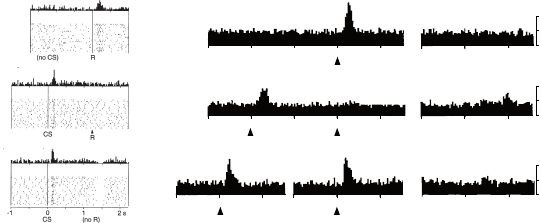
In one set of experiments, the dopaminergic (DA) neurons of macaque mon-
keys were recorded as they learned that a light is predictive of the availability
of a reward (juice, received by pressing a lever).
82
In the absence of reward,
DA neurons exhibit a sustained level of activity, given by the baseline or tonic
firing rate. Prior to learning, when a reward was delivered, the monkeys’ DA
neurons showed a sudden, short burst of activity, known as phasic firing (Figure
11.2a, top). After learning, the DA neurons’ firing rate no longer deviated from
the baseline when receiving the reward (Figure 11.2a, middle). However, pha-
sic activity was now observed following the appearance of the cue (CS, for
conditional stimulus).
One interpretation for these learning-dependent increases in firing rate is
that they encode a positive prediction error. The increase in firing rate at the
appearance of the cue, in particular, gives evidence that the cue itself eventually
induces a reward-based prediction error (RPE). Even more suggestive of an
error-driven learning process, omitting the juice reward following the cue
resulted in a decrease in firing rate (a negative prediction error) at the time at
which a reward was previously received; simultaneously, the cue still resulted
in an increased firing rate (Figure 11.2a, bottom).
The RPE interpretation was further extended when Montague et al. (1996)
showed that temporal-difference learning predicts the occurrence of a partic-
ularly interesting phenomenon found in an early experiment by Schultz et
al. (1993). In this experiment, macaque monkeys learned that juice could be
obtained by pressing one of two levers in response to a sequence of colored
lights. One of two lights (green, the “instruction”) first indicated which lever to
press. Then, a second light (yellow, the “trigger”) indicated when to press the
lever and thus receive an apple juice reward – effectively providing a first-order
cue.
Figure 11.2b shows recordings from DA neurons after conditioning. When
the instruction light was provided at the same time as the trigger light, the
DA neurons responded as before: positively in response to the cue. When the
instruction occurred consistently one second before the trigger, the DA neurons
showed an increase in firing only in response to the earlier of the two cues.
However, when the instruction was provided at a random time prior to the
trigger, the DA neurons now increased their firing rate in response to both
events – encoding a positive error from receiving the unexpected instruction
and the necessary error from the unpredictable trigger. In conclusion, varying
the time interval between these two lights produced results that could not be
82.
For a more complete review of reinforcement learning models of dopaminergic neurons and
experimental findings, see Schultz (2002), Glimcher (2011), and Daw and Tobler (2014).
Draft version.
326 Chapter 11
No prediction
Reward occurs
Reward predicted
Reward occurs
Reward predicted
No reward occurs
(a) (b)
//
//
//
//
10
5
0
imp/s
10
5
0
imp/s
10
5
0
imp/s
Instruction Trigger
-0.5 0.5 2.5 3.0 -0.5 0.5 s
03.5 s
0
Instruction Trigger
-0.5 0 0.5 1.0 -0.5 0.5 s
01.5 s
Instruction + Trigger
-1.5 -1.0 0.5 0 -0.5 0.5 s
00.5 s
Figure 11.2
(a)
DA activity when an unpredicted reward occurs, when a cue predicts a reward and it
occurs, and when a cue predicts a reward but it is omitted. The data are presented both
in raster plots showing firing of a single dopaminergic neuron and as peri-stimulus time
histograms (PSTHs) – histograms capturing neuron firing rate over time. Conditioned
stimulus (CS) marks the onset of the cue, with delivery or omission of reward indicated
by (R) or (no R). From Schultz et al. (1997). Reprinted with permission from AAAS.
(b)
PSTHs averaged over a population of dopamine neurons for three conditions examining
temporal credit assignment. From Schultz et al. (1993), copyright 1993 Society for
Neuroscience.
completely explained by the Rescorla–Wagner model but were consistent with
TD learning.
The temporal-difference learning model of dopaminergic neurons suggests
that, in aggregate, these neurons modulate their firing rate in response to unex-
pected rewards or in response to an anticipated reward failing to appear. In
particular, the model makes two predictions: first, that deviations from the
tonic firing rate should be proportional to the magnitude of the prediction error
(because the TD error in Equation 11.2 is linear in
r
), and second, that the tonic
firing rate in a trained animal should correspond to the situation in which the
received reward matches the expected value (that is,
r
+
γV
0
=
V
, in which case
there is no prediction error).
For a given DA neuron, let us call reversal point the amount of reward
r
0
for which, if a reward
r < r
0
is received, the neuron expresses a negative error,
and if a reward
r > r
0
is received, it expresses a positive error.
83
Under the
TD learning model, individual neurons should show approximately identical
reversal points (up to an estimation error) and should weigh positive and neg-
ative errors equally (Figure 11.3a). However, experimental evidence suggests
83.
Assuming that the return is
r
(i.e., there is no future value
V
0
). We can more generally define
the reversal point with respect to an observed return, but this distinction is not needed here.
Draft version.
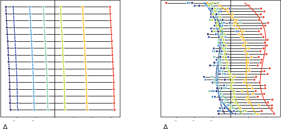
Two Applications and a Conclusion 327
3 2 1 0 1 2
Firing Rate (variance normalized)
Cell (Sorted by reversal point)
1.0 0.5 0.0 0.5 1.0 1.5
Firing Rate (variance normalized)
Cell (Sorted by reversal point)
(a) (b)
Figure 11.3
(a)
The temporal-difference learning model of DA neurons predicts that, while individual
neurons may show small variations in reversal point (e.g., due to estimation error), their
response should be linear in the TD error and weight positive and negative errors
equally. Neurons are sorted from top to bottom in decreasing order of reversal point.
(b)
Measurements of the change in firing rate in response to each of the seven possible reward
magnitudes (indicated by colour) for individual dopaminergic neurons in mice (Eshel
et al. 2015), sorted in decreasing order of imputed reversal point. These measurements
exhibit marked deviation from the linear error-response predicted by the TD learning
model.
otherwise – that individual neurons instead respond to the same cue in a man-
ner specific to each neuron and asymmetrically depending on the reward’s
magnitude (Figure 11.3b).
Eshel et al. (2015) measured the firing rate of individual DA neurons of
mice in response to a random reward 0
.
1
,
0
.
3
,
1
.
2
,
2
.
5
,
5
,
10, or 20
µ
L of juice,
chosen uniformly at random for each trial. Figure 11.4a shows the change
in firing rate in response to each reward, after conditioning, as a function of
each neuron’s imputed reversal point (see Dabney et al. 2018 for details). The
analysis illustrates a marked asymmetry in the response of individual neurons
to reward; the neurons with the lowest reversal points, in particular, increase
their firing rate for almost all rewards.
We may explain this phenomenon by considering a per-neuron update rule
that incorporates an asymmetric step size, known as the distributional TD model.
Because the neurons’ change in firing rate does in general vary monotonically
with the magnitude of the reward, it is natural to consider an incremental
algorithm derived from expectile dynamic programming (Section 8.6). As
before, let (
τ
i
)
m
1=1
be values in the interval (0
,
1), and (
θ
i
)
m
i=1
a set of adjustable
locations. Here,
i
corresponds to an individual DA neuron, such that
θ
i
denotes
Draft version.
328 Chapter 11
the predicted future reward for which this neuron computes an error, and
τ
i
determines the asymmetry in its step size. For a sample reward
r
, the negative
gradient of the expectile loss (Equation 8.13) with respect to
θ
i
yields the update
rule
θ
i
←θ
i
+ α |
{r < θ
i
}
−τ
i
|(r −θ
i
)
| {z }
expectile error
, (11.3)
Here, the term |
{r < θ
i
}
−τ
i
| constitutes an asymmetric step size.
Under this model, the reversal point of a neuron corresponds to the prediction
θ
i
, and therefore a neuron’s deviation from its tonic firing rate corresponds to
the expectile error. In turn, the slope or rate at which the firing rate is reduced
or increased as a function of the error reflects in some sense the neuron’s “step
size”
α|
{g < θ
i
}
−τ
i
|
. By measuring the slope of a neuron’s change in firing rate
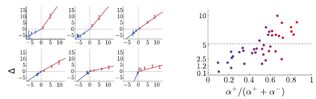
for rewards smaller and larger than the imputed reversal point, one finds that
different neurons indeed exhibit asymmetric slopes around their reversal point
(Figure 11.4a).
Given the slopes
α
+
and
α
−
above and below the reversal point, respectively,
for an individual neuron, we can recover an estimate of the asymmetry parameter
τ
i
according to
τ
i
=
α
+
α
+
+ α
−
.
With this change of variables, one finds a strong correlation between indi-
vidual neurons’ reversal points (
θ
i
) and their inferred asymmetries (
τ
i
); see
Figure 11.4b. This gives evidence that the diversity in responses to rewards of
different magnitudes is structured consistent with an expectile representation of
the distribution learned through asymmetric scaling of prediction errors, that is,
evidence supporting the distributional TD model of dopamine.
As a whole, these results suggest that the behavior of dopaminergic neurons
is best modeled not with a single global update rule, such as in TD learning,
but rather a collection of update rules that together describe a richer prediction
about future rewards – a distributional prediction. While the downstream uses
of such a prediction remain to be identified, one can naturally imagine that
there should be behavioral correlates involving risk and uncertainty. Other open
questions around distributional RL in the brain include: What are the biological
mechanisms that give rise to the diverse asymmetric responses in DA neurons?
How, and to what degree, are DA neurons and those that encode reversal points
coupled, as required by the distributional TD model? Does distributional RL
confer representation learning benefits in biological agents as it does in artificial
agents?
Draft version.
Two Applications and a Conclusion 329
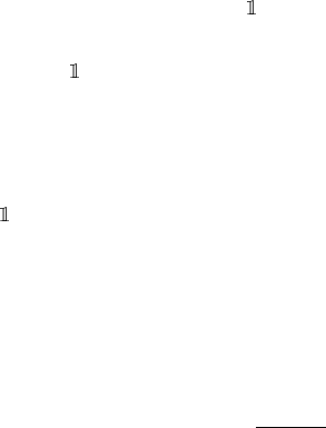
Reward minus reversal point
Firing Rate
Reversal point
(a) (b)
Figure 11.4
(a)
Examples of the change in firing rate in response to various reward magnitudes for
individual dopaminergic (DA) neurons showing asymmetry about the reversal point.
Each plot corresponds to an individual DA neuron, and each point within, with error bars
showing standard deviation over trials, shows that neuron’s change in firing rate upon
receiving one of the seven reward magnitudes. Solid lines correspond to the piecewise
linear best fit around the reversal point.
(b)
Estimated asymmetries strongly correlate
with reversal points as predicted by distributional TD. For all measured DA neurons
(
n
= 40), we show the estimated reversal point versus the cell’s asymmetry. We observe a
strong positive correlation between the two, as predicted by the distributional TD model.
11.3 Conclusion
The act of learning is fundamentally an anticipatory activity. It allows us to
deduce that eating certain kinds of foods might be hazardous to our health and
consequently avoid them. It helps the footballer decide how to kick the ball into
the opposite team’s net and the goalkeeper to prepare for the save before the
kick is even made. It informs us that studying leads to better grades; experience
teaches us to avoid the highway at rush hour. In a rich, complex world, many
phenomena carry a part of unpredictability, which in reinforcement learning
we model as randomness. In that respect, learning to predict the full range of
possible outcomes – the return distribution – is only natural: it improves our
understanding of the environment “for free,” in the sense that it can be done in
parallel with the usual learning of expected returns.
For the authors of this book, the roots of the distributional perspective lie
in deep reinforcement learning, as a technique for obtaining more accurate
representations of the world. By now, it is clear that this is but one potential
application. Distributional reinforcement learning has proven useful in settings
far beyond what was expected, including to model the behaviors of coevolving
agents and the dynamics of dopaminergic neurons. We expect this trend to
continue and look forward to seeing its greater application in mathematical
Draft version.
330 Chapter 11
finance, engineering, and life sciences. We hope this book will provide a sturdy
foundation on which these ideas can be built.
11.4 Bibliographical Remarks
11.1.
Game theory and the study of multiagent interactions is a research disci-
pline that dates back almost a century (von Neumann 1928; Morgenstern and
von Neumann 1944). Shoham and Leyton-Brown (2009) provide a modern
summary of a wide range of topics relating to multiagent interactions, and
Oliehoek and Amato (2016) provide a recent overview from a reinforcement
learning perspective. The MMDP model described here was introduced by
Boutilier (1996), and forms a special case of the general class of Markov games
(Shapley 1953; van der Wal 1981; Littman 1994). A commonly encountered
generalization of the MMDP is the Dec-POMDP (Bernstein et al. 2002), which
also allows for partial observations of the state. Lauer and Riedmiller (2000)
propose an optimistic algorithm with convergence guarantees in deterministic
MMDPs, and many other (nondistributional) approaches to decentralized con-
trol in MMDPs have since been considered in the literature (see, e.g., Bowling
and Veloso 2002; Panait et al. 2003; Panait et al. 2006; Matignon et al. 2007,
2012; Wei and Luke 2016), including in combination with deep reinforcement
learning (Tampuu et al. 2017; Omidshafiei et al. 2017; Palmer et al. 2018;
Palmer et al. 2019). There is some overlap between certain classes of these
techniques and distribution reinforcement learning in stateless environments,
as noted by Rowland et al. (2021), on which the distributional example in this
section is based.
11.2.
A thorough review of the research surrounding computational models
of DA neurons is beyond the scope of this book. For the machine learning
researcher, Niv (2009) and Sutton and Barto (2018) provide a broad discus-
sion and historical account of the connections between neuroscience and
reinforcement learning; see also the primer by Ludvig et al. (2011) for a
concise introduction to the topic and the work by Daw (2003) for a neuroscien-
tific perspective on computational models. Other recent, neuroscience-focused
overviews are provided by Shah (2012), Daw and Tobler (2014), and Lowet
et al. (2020). Here we highlight a few key works due to their historical rele-
vance, as well as those that provide context into both compatible and competing
hypotheses surrounding dopamine-based learning in the brain.
As discussed in Section 11.2, Montague et al. (1996) and Schultz et al. (1997)
provided the early experimental findings that led to the formulation of the
temporal-difference model of dopamine. These results followed mounting evi-
dence of limitations in the Rescorla–Wagner model (Schultz 1986; Schultz and
Romo 1990; Ljungberg et al. 1992; Miller et al. 1995).
Draft version.
Two Applications and a Conclusion 331
Dopamine’s role in learning (White and Viaud 1991), motivation (Mogenson
et al. 1980; Cagniard et al. 2006), motor control (Barbeau 1974), and attention
(Nieoullon 2002) has been extensively studied and we recommend the interested
reader consult Wise (2004) for a thorough review.
We arrived at our claim of less than 0
.
001 percent of the brain’s neurons
being dopaminergic based upon the following two results. First, there are
approximately 86
±
8 billion neurons in the adult human brain (Azevedo et
al. 2009), with only 400,000 to 600,000 dopaminergic neurons in the midbrain,
which itself contains approximately 75 percent of all DA neurons in the human
brain (Hegarty et al. 2013).
Much of the work untangling the role of DA in the brain was borne out of
studying associated neurological disorders. The loss of midbrain DA neurons is
seen as the neurological hallmark of Parkinson’s disease (Hornykiewicz 1966;
German et al. 1989), while ADHD is associated with reduced DA activity
(Olsen et al. 2021), and the connections between dysregulation of the dopamine
system and schizophrenia have continued to be studied and refined for many
years (Braver et al. 1999; Howes and Kapur 2009).
Recently, Muller et al. (2021) used distributional RL to model reward-related
responses in the prefrontal cortex (PFC). This may suggest a more ubiquitous
role for distributional RL in the brain.
While the distributional TD model posits that DA neurons differ in their
sensitivity to positive versus negative prediction errors, several alternative
models have been proposed to explain the observed diversity in dopaminergic
response. Kurth-Nelson and Redish (2009) propose that the brain encodes value
with a distributed representation over temporal discounts, with a multitude of
value prediction channels differing in their discount factor. Such a model can
readily explain observations of purported hyperbolic discounting in humans
and animals. We also note that these neuroscientific models have themselves
inspired recent work in deep RL that combines multiple discount factors and
distributional predictions (Fedus et al. 2019).
Another line of research proposes to generalize temporal-difference learning
to prediction errors over reward-predictive features (Schultz 2016; Gardner et
al. 2018). These are motivated by findings in neuroscience, which have shown
that DA neurons may increase their firing in response to unexpected changes
in sensory features, independent of anticipated reward (Takahashi et al. 2017;
Stalnaker et al. 2019). This generalization of the TD model is grounded in
the concept of successor representations (Dayan 1993), but is perhaps more
precisely characterized as successor features (Barreto et al. 2017), where the
features are themselves predictive of reward.
Draft version.
332 Chapter 11
Tano et al. (2020) propose a temporal-difference learning algorithm for distri-
butional reinforcement learning which uses a variety of discount factors, reward
sensitivities, and multistep updates, allowing the population to make distribu-
tional predictions with a linear operator. The advantage of such a model is that it
is local, in the sense that there need not be any communication between the var-
ious value prediction channels, whereas distributional TD assumes significant
communication among the DA neurons. Relatedly, Chapman and Kaelbling
(1991) consider estimating the value function by decomposing it into the total
discounted probability of individual reward outcomes.
Draft version.