10
Deep Reinforcement Learning
As a computational description of how an organism learns to predict, temporal-
difference learning reduces the act of learning, prediction, and control to
numerical operations and mostly ignores how the inputs and outputs to these
operations come to be. By contrast, real learning systems are but a component
within a larger organism or machine, which in some sense provides the inter-
face between the world and the learning component. To understand and design
learning agents, we must also situate their computational operations within a
larger system.
In recent years, deep reinforcement learning has emerged as a framework
that more directly studies how characteristics of the environment and the archi-
tecture of an artificial agent affect learning and behavior. The name itself comes
from the combination of reinforcement learning techniques with deep neural
networks, which are used to make sense of low-level perceptual inputs, such
as images, and also structure complex outputs (such as the many degrees of
freedom of a robotic arm). Many of reinforcement learning’s recent applied
successes can be attributed to this combination, including superhuman perfor-
mance in the game of Go, robots that learn to grasp a wide variety of objects,
champion-level backgammon play, helicopter control, and autonomous balloon
navigation.
Much of the recent research in distributional reinforcement learning, includ-
ing our own, is rooted in deep reinforcement learning. This is no coincidence,
since return distributions are naturally complex objects, whose learning is facil-
itated by the use of deep neural networks. Conversely, predicting the return also
translates into practical benefits, often in the guise of accelerated and more sta-
ble learning. In this context, the distributional method helps the system organize
its inputs into features that are useful for further learning, a process known as
representation learning. This chapter surveys some of these ideas and discusses
practical considerations in introducing distributional reinforcement learning to
a larger-scale system.
Draft version. 293
294 Chapter 10
Replay Buffer
Periodically
Updated
Target Network
Online Network
Pre-processing Convolutional Layers Fully-connected Layers
(a) (b)
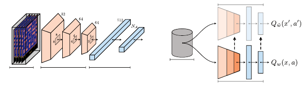
Figure 10.1
(a)
The deep neural network at the heart of the DQN agent architecture. The network
takes as inputs four preprocessed images and outputs the predicted state-action value
estimates.
(b)
The replay buffer provides the sample transitions used to update the main
(online) network (Equation 10.2). A second target network is used to construct sample
targets and is periodically updated with the weights of the online network. Example input
to the network is visualized with frames from the Atari game Ms. Pac-Man (published
by Midway Manufacturing).
10.1 Learning with a Deep Neural Network
The term deep neural network (or simply deep network) designates a fairly
broad class of functions built from a composition of atomic elements (called
neurons or hidden units), typically organized in layers and parameterized by
weight vectors and one or many activation functions. The function’s inputs
are transformed by the first layer, whose outputs become the inputs of the
second layer, and so on. Canonically, the weights of the network are adjusted to
minimize a given loss function by gradient descent. In that respect, one may
view linear function approximation as a simple neural network architecture that
maps inputs to outputs by means of a single, nonadjustable layer implementing
the chosen state representation.
More sophisticated architectures include: convolutional neural networks
(LeCun and Bengio 1995), particularly suited to learning functions that exhibit
some degree of translation invariance; recurrent networks (Hochreiter and
Schmidhuber 1997), designed to deal with sequences; and attention mechanisms
(Bahdanau et al. 2015; Vaswani et al. 2017). The reader interested in further
details is invited to consult the work of Goodfellow et al. (2016).
By virtue of their parametric flexibility, deep neural networks have proven
particularly effective at dealing with reinforcement learning problems with
high-dimensional structured inputs. As an example, the DQN algorithm (Deep
Q-Networks; Mnih et al. 2015) applies the tools of deep reinforcement learning
to achieve expert-level game play in Atari 2600 video games. More properly
speaking, DQN is a system or agent architecture that combines a deep neural
Draft version.
Deep Reinforcement Learning 295
network with a semi-gradient Q-learning update rule and a few algorithmic
components that improve learning stability and efficiency. DQN also contains
subroutines to transform received observations into a useful notion of state and
to select actions to be enacted in the environment. We divide the computation
performed by DQN into four main subtasks:
(a) preprocessing observations (Atari 2600 images) into an input vector,
(b) predicting future outcomes given such an input vector,
(c) behaving on the basis of these predictions, and finally
(d) learning to improve the agent’s predictions from its experience.
Preprocessing.
The Arcade Learning Environment or ALE (Naddaf 2010;
Bellemare et al. 2013a) provides a reinforcement learning interface to the Stella
Atari 2600 emulator (Mott et al. 1995–2023). This interface produces 210
×
160,
7-bit pixel images in response to one of eighteen possible joystick motions
(combinations of an up-down motion, a left-right motion, and a button press). A
single emulation step or frame lasts 1
/
60th of a second, but the agent only selects
a new action every four frames, what might be more appropriately called a
time step (that is, fifteen times per emulated second; for further implementation
details, see Machado et al. (2018)).
In order to simplify the learning process and make it more suitable for rein-
forcement learning, DQN transforms or preprocesses the images and rewards it
receives from the ALE. Every time step, the DQN agent converts the most recent
frame to 7-bit grayscale (preserving luminance). It combines this frame with
the immediately preceding one, similarly converted, by means of a max-pooling
operation that takes the pixel-wise maximum of the two images. The result
is then downscaled to a smaller 84
×
84 size, and pixel values are normalized
from 0 (black) to 1 (white). The four most recent images (spanning a total of 16
frames, a little over 1
/
4th of a second) are concatenated together to form the
input vector, of size 84
×
84
×
4.
74
In essence, DQN uses this input vector as a
surrogate for the state x.
The Arcade Learning Environment also provides an integer reward indicating
the change in score (positive or negative) between consecutive time steps. DQN
applies an operation called reward clipping, which keeps only the sign of the
provided reward (−1, 0, or 1). The result is what we denote by r.
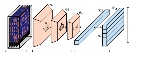
Prediction.
DQN uses a five layer neural network to predict the expected
return from the agent’s current state (see Figure 10.1a). The network’s input is
the stack of frames produced by the preprocessor. This input is successively
74.
In many games, these images do not provide a complete picture of the game state. In this case,
the problem is said to be partially observable. See, for example, Kaelbling et al. (1998).
Draft version.
296 Chapter 10
transformed by three convolutional layers that extract features from the image,
and then by a fully connected layer that applies a linear transformation and
a nonlinearity to the output of the final convolutional layer. The result is a
512-dimensional vector, which is then linearly transformed into
N
A
= 18 values
corresponding to the predicted expected returns for each action. If we denote by
w
the entire collection of weights of the neural network, then the approximation
Q
w
(
x, a
) denotes the resulting prediction made by DQN. Here,
x
is described by
the input image stack and
a
indexes into the network’s
N
A
-dimensional output
vector.
Behavior and experience.
DQN acts according to an
ε
-greedy policy derived
from its approximation
Q
w
. More precisely, this policy assigns 1
−ε
of its
probability mass to a greedy selection rule that breaks ties uniformly at random.
Provided that
Q
w
assigns a higher value to better actions, acting greedily results
in good performance. The remaining
ε
probability mass is divided equally
among all actions, allowing for some exploration of unseen situations and
eventually improving the network’s value estimates from experience.
Similar to the online setting described by Algorithms 3.1 and 3.2, the sample
produced by the agent’s interactions with the Arcade Learning Environment is
used to improve the network’s value predictions (see
Learning
below). Here,
however, the transitions are not provided to the learning algorithm as they
are experienced but are instead stored in a circular replay buffer. The replay
buffer stores the last 1 million transitions experienced by the agent; as the
name implies, these are typically replayed multiple times as part of the learning
process. Compared to learning from each piece of experience once and then
discarding it, using a replay buffer has been empirically demonstrated to result
in greater sample efficiency and stability.
Learning.
Every four time steps, DQN samples a minibatch of thirty-two
sample transitions from its replay buffer, uniformly at random. As with linear
approximation, these sample transitions are used to adjust the network weights
w
with a semi-gradient update rule. Given a second target network with weights
˜w and a sample transition (x, a, r, x
0
), the corresponding sample target is
r + γ max
a
0
∈A
Q
˜w
(x
0
, a
0
) . (10.1)
Canonically, the discount factor is chosen to be γ = 0.99.
In deep reinforcement learning, the update to the network’s parameters is
typically expressed first and foremost in terms of a loss function
L
to be
minimized. This is because automatic differentiation can be used to efficiently
compute the gradient
∇
w
L
(
w
) by means of the backpropagation algorithm
(Werbos 1982; Rumelhart et al. 1986). In the case of DQN, the sample target is
Draft version.

Deep Reinforcement Learning 297
used to construct the squared loss
L(w) =
r + γ max
a
0
∈A
Q
˜w
(x
0
, a
0
) −Q
w
(x, a)
2
.
Taking the gradient of
L
with respect to
w
, we obtain the semi-gradient update
rule:
w ←w + α
r + γ max
a
0
∈A
Q
˜w
(x
0
, a
0
) −Q
w
(x, a)
∇
w
Q
w
(x, a) . (10.2)
In practice, the actual loss to be minimized is the average loss over the sampled
minibatch. Consequently, the semi-gradient update rule adjusts the weight vector
on the basis of all sampled transitions simultaneously. After a specified number
of updates have been performed (10,000 in the original implementation), the
weights
w
of the main network (also called online network) are copied over to
the target network; the process is illustrated in Figure 10.1b. As discussed in
Section 9.4, the use of a target network allows the semi-gradient update rule
to behave more like the projected Bellman operator and mitigates some of the
convergence issues of semi-gradient methods.
Equation 10.2 generalizes the semi-gradient rule for linear value function
approximation (Equation 9.11) to nonlinear schemes; observe that if
Q
w
(
x, a
) =
φ(x, a)
>
w, then
∇
w
Q
w
(x, a) = φ(x, a) .
In practice, more sophisticated adaptive gradient descent methods (see,
e.g., Tieleman and Hinton 2012; Kingma and Ba 2015) are used to accel-
erate convergence. Additionally, the Huber loss is a popular alternative to the
squared loss. For κ ≥0, the Huber error function is defined as
H
κ
(u) =
1
2
u
2
, if |u|≤κ
κ(|u|−
1
2
κ), otherwise .
DQN’s Huber loss instantiates this error function with κ = 1:
L(w) = H
1
r + γ max
a
0
∈A
Q
˜w
(x
0
, a
0
) −Q
w
(x, a)
.
The Huber loss corresponds to the squared loss for small errors but behaves like
the
L
1
loss for larger errors. In effect, this puts a limit on the magnitude of the
updates to the weight vector, which in turn reduces instability in the learning
process.
Viewed as an agent interacting with its environment, DQN operates by acting
in the world according to its state-action value function estimates, collecting new
experience along the way. It then uses this experience to produce an improved
policy that is used to collect better experience and so on. Given sufficient
training time, this approach can learn fairly complex behavior from pixels and
rewards alone, including behavior that exploits computer bugs in some of Atari
Draft version.
298 Chapter 10
Pre-processing Convolutional Layers Fully-connected Layers
Distribution
Parameters
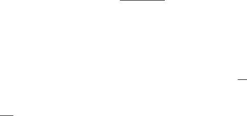
Figure 10.2
The extension of DQN to the distributional setting uses a deep neural network that outputs
m
distribution parameters per action. The same network architecture is used for both
C51 (categorical representation) and QR-DQN (quantile representation). Example input
to the network is visualized with frames from the Atari game Ms. Pac-Man (published
by Midway Manufacturing).
2600 games. Although it is possible to achieve the same behavior by using a
fixed state representation and learning a linear value approximation (Machado
et al. 2018), in practice, doing so without a priori knowledge of the specific
game being played is computationally demanding and eventually does not scale
as effectively.
10.2 Distributional Reinforcement Learning with Deep Neural
Networks
We extend DQN to the distributional setting by mapping state-action pairs to
return distributions rather than to scalar values. A simple approach is to change
the network to output one
m
-dimensional parameter vector per action (equiva-
lently, one
N
A
×m
-dimensional parameter matrix, as illustrated in Figure 10.2).
These vectors are then interpreted as the parameters of return distributions,
by means of a probability distribution representation (Section 5.2). The target
network is modified in the same way.
By making different choices of distribution representation or rule for updat-
ing the parameters of these distributions, we obtain different distributional
algorithms. The C51 algorithm, in particular, is based on the categorical repre-
sentation, while the QR-DQN algorithm is based on the quantile representation.
Their respective update rules follow those of linear CTD and linear QTD in
Section 9.5, and here we emphasize the differences from the linear approach.
We begin with a description of the C51 algorithm.
Draft version.
Deep Reinforcement Learning 299
Prediction.
C51 owes its name to its use of a 51-categorical representation
in its original implementation (Bellemare et al. 2017a), but the name generally
applies for any such agent with
m ≥
2. Given an input state
x
, its network outputs
a collection of softmax parameters ((ϕ
i
(x, a))
m
i=1
: a ∈A). These parameters are
used to define the state-action categorical distributions:
η
w
(x, a) =
m
X
i=1
p
i
(x, a; w)δ
θ
i
,
where p
i
(x, a; w) is a probability given by the softmax distribution:
p
i
(x, a; w) =
e
ϕ
i
(x,a;w)
m
P
j=1
e
ϕ
j
(x,a;w)
.
The standard implementation of C51 parameterizes the locations
θ
1
, . . . , θ
m
in
two specific ways: first,
θ
1
and
−θ
m
are chosen to be negative of each other,
so that the support of the distribution is symmetric around 0. Second, it is
customary to take
m
to be an odd number so that the central location
θ
m−1
2
is zero.
The canonical choice is
θ
1
=
−
10 and
θ
m
= 10; we will study the effect of this
choice in Section 10.4. Even though the largest theoretically achievable return
is
V
max
=
R
max
1−γ
= 100, the choice of
θ
m
= 10 is sensible because in most Atari
2600 video games, the player’s score only changes infrequently. Consequently,
the reward is zero on most time steps and the largest return actually observed
is typically much smaller than the analytical maximum (the same argument
applies to V
min
and θ
1
).
Behavior.
C51 is designed to optimize for the risk-neutral objective. The
value function induced by its distributional predictions is
Q
w
(x, a) = E
Z∼η
w
(x,a)
[Z] =
m
X
i=1
p
i
(x, a; w)θ
i
,
and similarly for
Q
˜w
. The agent acts according to an
ε
-greedy policy defined
from the main network’s state-action value estimates Q
w
(x, a).
Learning.
The sample target is obtained from the combination of an update
and projection step. Following Section 9.5, given a transition (
x, a, r, x
0
), the
sample target is given by
¯η(x, a) =
m
X
j=1
¯p
j
δ
θ
j
= Π
c
(b
r,γ
)
#
η
˜w
(x
0
, a
˜w
(x
0
))
,
where
a
˜w
(x
0
) = arg max
a
0
∈A
Q
˜w
(x
0
, a
0
)
Draft version.
300 Chapter 10
is the greedy action for the induced state-action value function
Q
˜w
. As in the
linear setting, this sample target is used to formulate a cross-entropy loss to be
minimized (Equation 9.18):
L(w) = −
m
X
j=1
¯p
j
log p
j
(x, a; w) .
Updating the parameters
w
in the direction of the negative gradient of this loss
yields the (first-order) semi-gradient update rule
w ←w + α
m
X
i=1
¯p
i
− p
i
(x, a; w)
∇
w
θ
i
(x, a; w) .
It is useful to contrast the above with the linear CTD semi-gradient update rule
(Equation 9.19):
w
i
←w
i
+ α
¯p
i
− p
i
(x, a; w)
φ(x, a) .
With linear CTD, the update rule takes a simple form where one computes the
per-particle categorical TD error
˜p
i
− p
i
(
x, a
;
w
)
and moves the weight vector
w
i
in the direction
φ
(
x, a
) in proportion to this error. This is possible because
the softmax parameters
ϕ
i
(
x, a
;
w
) =
φ
(
x, a
)
>
w
i
are linear in
φ
and consequently
∇
w
i
ϕ
i
(x, a; w) = φ(x, a) ,
similar to the value-based setting. When using a deep network, however, the
weights at earlier layers affect the entire predicted distribution and it is not
possible to perform per-particle weight updates independently.
QR-DQN.
QR-DQN uses the same neural network as C51 but interprets
the output vectors as parameters of a
m
-quantile representation, rather than a
categorical representation:
η
w
(x, a) =
1
m
m
X
i=1
δ
θ
i
(x,a;w)
.
Its induced value function is simply
Q
w
(x, a) =
1
m
m
X
i=1
θ
i
(x, a; w) .
Given a sample transition (
x, a, r, x
0
) and levels
τ
1
, . . . , τ
m
, the parameters are
updated by performing gradient descent on the Huber quantile loss
L(w) =
1
m
m
X
i, j=1
ρ
H
τ
i
r + γθ
j
(x
0
, a
˜w
(x
0
); ˜w) −θ
i
(x, a; w)
,
where ρ
H
τ
(u) = |
{u < 0}
−τ|H
1
(u) .
Draft version.
Deep Reinforcement Learning 301
The Huber quantile loss behaves like the quantile loss (Equation 6.12) for
large errors but like the expectile loss (the single-sample equivalent of Equa-
tion 8.13) for sufficiently small errors. This loss is minimized by a statistical
functional between a quantile and expectile. The Huber quantile loss can be
interpreted as a smoothed version of the quantile regression loss (Sections 6.4
and 9.5), which leads to more stable behavior when combined with the nonlinear
function approximation and adaptive gradient descent methods used in deep
reinforcement learning.
10.3 Implicit Parameterizations
The value function
Q
π
can be viewed as a mapping from state-action pairs to
real values. When there are finitely many actions and the state space is small
and finite, a tabular representation of this mapping is usually sufficient – in
this case, each entry in the table corresponds to the value at a given state and
action. Much like linear function approximation, neural networks improve on
the tabular representation by parameterizing the relationship between similar
states, allowing us to generalize the learned function to unseen states. It is
therefore useful to think of the inputs of DQN’s neural network as arguments
to a function and its outputs as the evaluation of this function. Under this
perspective, the network implements a function mapping
X
to
R
A
, which can
be interpreted as the function
Q
w
:
X×A→R
by a further indexing into the
output vector.
Similarly, we can represent probability distributions as different kinds of
functions. For example, the probability density function
f
ν
of a suitable distri-
bution
ν ∈P
(
R
) is a mapping from
R
to [0
, ∞
) and its cumulative distribution
is a monotonically increasing function from
R
to [0
,
1]. A distribution can also
be represented by its inverse cumulative distribution function
F
−1
ν
: (0
,
1)
→R
,
which we call quantile function in the context of this section. By extension,
a state-action return function can be viewed as a function of three arguments:
x ∈X
,
a ∈A
, and a distribution parameter
τ ∈
(0
,
1). That is, we may represent
η by the mapping
(x, a, τ) 7→F
−1
η(x,a)
(τ) .
Doing so gives rise to an implicit approach to distributional reinforcement
learning, which makes the distribution parameter an additional input to the
network.
To understand this idea, it is useful to contrast it with the two algorithms of
the previous section. Both C51 and QR-DQN take a half-and-half approach: the
state
x
is provided as input to the network, but the parameters of the distribution
(the probabilities
p
i
or locations
θ
i
, accordingly) are given by the network’s
Draft version.
302 Chapter 10
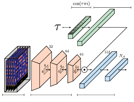
Pre-processing Convolutional Layers Fully-connected Layers
Fully-connected Layer
Figure 10.3
The deep neural network used by IQN. IQN outputs a single scalar per action, corre-
sponding to the queried
τ
th quantile. The input
τ
to the network is encoded using a
cosine embedding and multiplicatively combined with one of the network’s inner layers
(see Remark 10.1). Example input to the network is visualized with frames from the
Atari game Ms. Pac-Man (published by Midway Manufacturing).
outputs, one m-dimensional vector per action. This is conceptually simple and
has the advantage of leveraging probability distribution representations whose
behavior is theoretically well understood in the tabular setting. On the other
hand, the implied discretization of the return distributions incurs some cost,
for example, due to diffusion (Section 5.8). If instead we turn the distribution
parameter into an input to the network, we gain the benefits of generalization,
and in principle we can learn an approximation to the return function that is
only limited by the capacity of the neural network.
Prediction.
The implicit quantile network (IQN) algorithm instantiates the
argument-as-inputs principle by parameterizing the quantile function within
the neural network (Figure 10.3). As before, one of the network’s inputs is a
description of the state
x
: in the case of a DQN-type architecture, the stack
of preprocessed Atari 2600 images. In addition, the network also receives as
input a desired level
τ ∈
(0
,
1). This level is encoded by the cosine embedding
ϕ(τ) ∈R
M
:
ϕ(τ) = (cos(πτi))
M−1
i=0
.
In effect, the cosine embedding represents
τ
as a real-valued vector, making
it easier for the neural network to work with. The network’s output is an
N
A
-
dimensional vector describing the evaluation of the quantile function
F
−1
η(x,a)
(
·
)
Draft version.

Deep Reinforcement Learning 303
at this
τ
. With this construction, the neural network outputs the approximation
θ
w
(x, a, τ) = φ
w
(x, τ)
>
w
a
≈F
−1
η(x,a)
(τ) ,
where
φ
w
(
x, τ
)
∈R
n
are learned features for the (
x, τ
) pair and
w
a
∈R
n
are per-
action weights. Remark 10.1 provides details on how
φ
w
(
x, τ
) is implemented
in the network.
Behavior.
Because IQN represents the quantile function implicitly, the
induced state-action value functions
Q
w
and
Q
˜w
are approximated by a sam-
pling procedure, where as before
˜w
denotes the weights of the target network.
This approximation is obtained by drawing
m
levels
τ
1
, . . . , τ
m
uniformly and
independently from the (0
,
1) interval and averaging the output of the network
at these levels:
Q
w
(x, a) ≈
1
m
m
X
i=1
θ
w
(x, a, τ
i
) . (10.3)
As with the other algorithms presented in this chapter, IQN acts according to an
ε-greedy policy derived from Q
w
, with greedy action a
w
(x).
Learning.
Where QR-DQN aims to learn the quantiles of the return distri-
bution at a finite number of fixed levels, IQN aims to approximate the entire
quantile function of this distribution.
75
Because each query to the network
returns the network’s prediction evaluated for a single level, learning proceeds
somewhat differently. First, a pair of levels
τ
and
τ
0
is sampled uniformly from
(0
,
1). These determine the level at which the quantile function is to be updated
and a level from which a sample target is constructed. For a given sample
transition (x, a, r, x
0
) and levels τ, τ
0
, the two-sample IQN loss is
L
τ,τ
0
(w) = ρ
H
τ
r + γθ
˜w
(x
0
, a
˜w
(x
0
), τ
0
) −θ
w
(x, a, τ)
.
The variance of the sample gradient of this loss is reduced by averaging the
two-sample loss over many pairs of levels τ
1
, . . . , τ
m
1
and τ
0
1
, . . . , τ
0
m
2
:
L(w) =
1
m
2
m
1
X
i=1
m
2
X
j=1
L
τ
i
,τ
0
j
(w) .
Risk-sensitive control.
An appealing side effect of using an implicit param-
eterization is that many risk-sensitive objectives can be computed simply by
changing the sampling distribution for Equation 10.3. For example, given a pre-
dicted quantile function
θ
w
(
x, a, ·
) with instantiated random variable
G
w
(
x, a
),
recall that the CVaR of
G
w
(
x, a
) for a given level
¯τ ∈
(0
,
1) is, in the integral
75.
Of course, in practice, the predictions made by IQN might not actually correspond to the return
distribution of any fixed policy, because of approximation, bootstrapping, and issues arising in the
control setting (Chapter 7).
Draft version.
304 Chapter 10
form of Equation 7.20,
CVaR
¯τ
G
w
(x, a)
=
1
¯τ
Z
¯τ
0
θ
w
(x, a, τ)dτ .
Similar to the procedure for estimating the expected value of
G
w
(
x, a
) (Equation
10.3), this integral can be approximated by sampling
m
levels
τ
1
, . . . , τ
m
, but
now from the (0, ¯τ) interval:
CVaR
¯τ
G
w
(x, a)
≈
1
m
m
X
i=1
θ
w
(x, a, τ
i
), τ
i
∼U([0, ¯τ]) .
Treating the distribution parameter as a network input opens up the possibility
for a number of different algorithms, of which IQN is but one instantiation.
In particular, in problems where actions are real-valued (for example, when
controlling a robotic arm), it is common to also make the action
a
an input to
the network.
10.4 Evaluation of Deep Reinforcement Learning Agents
To illustrate the practical value of deep reinforcement learning and the added
benefits from predicting return distributions, let us take a closer look at how
well the algorithms presented in this chapter can learn to play Atari 2600 video
games. As the Arcade Learning Environment provides an interface to more
than sixty different games, a standard evaluation procedure is to apply the same
algorithm across a large set of games and report its performance on a per-game
basis, as well as aggregated across games (see Machado et al. 2018 for a more
complete discussion). Here, performance is measured in terms of the in-game
score achieved during one play-through (i.e., an episode). One particularly
attractive feature of Atari 2600 games, from a benchmarking perspective, is that
almost all games explicitly provide such a score. Measuring performance in
terms of game score has the additional advantage that it allows us to numerically
compare the playing skill of learning agents to that of human players.
The goal of the learning agent is to improve its performance at a given game
by repeatedly playing that game – in more formal terms, to optimize the risk-
neutral control objective from sample interactions.
76
The agent interacts with
the environment for a total of 200 million frames per game (about 925 hours of
game-play). Experimentally, we repeat this process multiple times in order to
evaluate the performance of the agent across different initial network weights
76.
Note, however, that the in-game score differs from the agent’s actual learning objective, which
involves a discount factor (canonically,
γ
= 0
.
99) and clipped rewards. This metric-objective mis-
match is well studied in the literature (e.g., van Hasselt et al. 2016a), and exists in part because
optimizing for the undiscounted, unclipped return with DQN produces unstable behavior.
Draft version.
Deep Reinforcement Learning 305
and realizations of the various sources of randomness. Following common
usage, we call each repetition a trial and the process itself training the agent.
Figure 10.4 (left) illustrates the overall progress made by DQN, C51, QR-DQN,
and IQN over the course these interactions, evaluated every 1 million frames.
Quantitatively, we measure an agent’s performance in terms of an aggregate
metric called human-normalized interquartile mean score (HNIQM), which we
now define.
Definition 10.1.
Denote by
g
the score achieved by a learning agent on a
particular game and by
g
h
and
g
r
the score achieved by two reference agents
(a human expert and the random policy). Assuming that
g
h
> g
r
, we define the
human-normalized score as
hns(g, g
h
, g
r
) =
g −g
r
g
h
−g
r
. 4
In the standard evaluation protocol described here, a learning agent’s perfor-
mance during training corresponds to its average per-episode score, measured
from 500,000 frames of additional, evaluation-only interactions with the
environment.
Definition 10.2.
Let
E
be a set of
E
games on which we have evaluated an
agent for
K
trials. For 1
≤k ≤ K
and
e ∈E
, denote by
s
k
e
the human-normalized
score achieved on trial k:
s
k
e
= hns (g
k
e
, g
h
e
, g
r
e
) ,
where
g
k
e
, g
h
e
, and
g
r
e
are respectively the agent’s, human player’s, and random
policy’s score on game
e
. Suppose that (
ˆs
i
)
K×E
i=1
denotes the vector of these
human-normalized scores, sorted so that
ˆs
i
≤ ˆs
i+1
, for all
i
= 1
, . . . , K ×E −
1.
The human-normalized interquartile mean score is given by
1
E
1
−E
0
E
1
−1
X
i=E
0
ˆs
i
, (10.4)
where E
0
is the integer nearest to
KE
4
and E
1
= KE −E
0
. 4
The normalization to human performance makes it possible to compare scores
across games; although it is also possible to evaluate agents in terms of their
mean or median normalized scores, these aggregates tend to be less representa-
tive of the full distribution of scores. As shown in Figure 10.4, it is accepted
practice (see, e.g., Agarwal et al. (2021)) to measure the degree of variability in
performance across trials and games using some empirically-determined confi-
dence interval. One should be mindful that such an interval, while informative,
does not typically guarantee statistical significance – for example, because there
are too few samples to aggregate or because these samples are not identically
Draft version.
306 Chapter 10
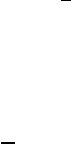
Figure 10.4
Top and bottom
: Evaluation using the deterministic-action and sticky-action versions of
the Arcade Learning Environment, respectively.
Left
: Human-normalized interquartile
mean score (HNIQM; see main text) across fifty-seven Atari 2600 games during the
course of learning. A normalized score of 1.0 indicates human-level performance, on
aggregate. Per-game scores were obtained from five independent trials for each algorithm
×
game configuration. Shading indicates bootstrapped 95 percent confidence intervals
(see main text).
Right
: Game scores obtained by different algorithms and a human
expert (dashed line); the scale of these scores is indicated at the top left of each graph;
dots indicate individual per-trial scores. The reported scores are measured at the end of
training.
distributed. Consequently, it is also generally recommended to report individual
game scores in addition to aggregate performance. Figure 10.4 (right) illustrates
this for a selected subset of games.
These results show that reinforcement learning, combined with deep neural
networks, can achieve a high level of performance on a wide variety of Atari
2600 games. Additionally, this performance improves with more training. This
is particularly remarkable given that the learning algorithm is only provided
game images as input, rather than game-specific features such as the location of
objects or the number of remaining lives. It is worth noting that although each
agent uses the same network architecture and hyperparameters
77
across Atari
2600 games, there are a few differences between the hyperparameters used by
77.
Following common usage, we use the term “hyperparameter” to distinguish the learned
parameters (e.g., w) from the parameters selected by the user (e.g., m and θ
1
, . . . , θ
m
).
Draft version.
Deep Reinforcement Learning 307
these agents; these differences match what is reported in the literature and are
the default choices in the code used for these experiments (Quan and Ostrovski
2020). The question of how to account for hyperparameters in scientific studies
is an active area of research (see, e.g., Henderson et al. 2018; Ceron and Castro
2021; Madeira Auraújo et al. 2021).
Historically, all four agents whose performance is reported here were trained
on what is called the deterministic-action version of the Arcade Learning Envi-
ronment, in which arbitrarily complicated joystick motions can be performed.
For example, nothing prevents the agent from alternating between the “left”
and “right” actions every four frames (fifteen times per emulated second). This
makes the comparison with human players somewhat unrealistic, as human play
involves a minimum reaction time and interaction with a mechanical device that
may not support such high-frequency decisions. In addition, some of the poli-
cies found by agents in the deterministic setting exploit quirks of the emulator
in ways that were clearly not intended by the designer.
To address this issue, more recent versions of the Arcade Learning Environ-
ment implement what is called sticky actions – a procedure that introduces a
variable delay in the environment’s response to the agent’s actions. Figure 10.4
(bottom panels) shows the results of the same experiment as above, but now
with sticky actions. The performance of the various algorithms considered here
generally remains similar, with some per-game differences (e.g., for the game
Space Invaders).
Although Atari 2600 games are fundamentally deterministic, randomness is
introduced in the learning process by a number of phenomena, including side
effects of distributional value iteration (Section 7.4), state aliasing (Section 9.1),
the use of a stochastic
ε
-greedy policy, and the sticky-actions delay added by the
Arcade Learning Environment. In many situations, this results in distributional
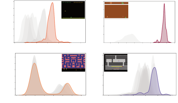
agents making surprisingly complex predictions (Figure 10.5). A common
theme is the appearance of bimodal or skewed distributions when the outcome
is uncertain – for example, when the agent’s behavior in the next few time steps
is critical to its eventual success or failure. Informally, we can imagine that
because the agent predicts such outcomes, it in some sense “knows” something
more about the state than, say, an agent that only predicts the expected return.
We will see some evidence to this effect in the next section.
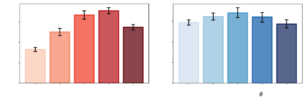
Furthermore, incorporating distributional predictions in a deep reinforcement
learning agent provides an additional degree of freedom in defining the number
and type of predictions that an agent makes at any given point in time. C51, for
example, is parameterized by the number of particles
m
used to represent prob-
ability distributions as well as the range of its support (described by
θ
m
). Figure
10.6 illustrates the change in human-normalized interquartile mean (measured
Draft version.
308 Chapter 10
11.5 12.0 12.5 13.0 13.5 14.514.0
Return
0.0
0.5
1.0
1.5
2.0
2.5
3.0
Density
17.5 20.0 22.5 25.0 27.5 30.0 32.5 35.0
Return
0.00
0.05
0.10
0.15
0.20
0.25
0.30
Density
0.5 0.6 0.7 0.8 0.9 1.0 1.1 1.2 1.3
Return
0
5
10
15
20
25
Density
1.0 1.5 2.0 2.5 3.0 3.5
Return
0
1
2
3
4
Density
(a)
(c)
(b)
(d)
Figure 10.5
Example return distributions predicted by IQN agents in four Atari 2600 games:
(a)
Space Invaders (published by Atari, Inc.),
(b)
Pong (from Video Olympics, published by
Atari, Inc.),
(c)
Ms. Pac-Man (published by Midway Manufacturing), and
(d)
H.E.R.O.
(published by Atari, Inc.). In each panel, action-return distributions for the game state
shown are estimated for each action using kernel density estimation (over 1000 samples
τ
). The outlined distribution corresponds to the action with the highest expected return
estimate (chosen by the greedy selection rule).
at the end of training) that results from varying both of these hyperparameters.
These results illustrate the commonly reported finding that predicting distribu-
tions leads to improved performance, with more accurate predictions generally
helping. More generally, this illustrates that an agent’s performance depends
to a good degree on the chosen distribution representation; this is an example
of what is called an inductive bias. In addition, as illustrated by the results for
m
= 201 and larger values of
θ
m
, there is clearly a complex relationship between
an agent’s parameterization and its aggregate performance across Atari 2600
games.
The development of deep distributional reinforcement learning agent architec-
tures continues to be an active area of research. Recent advances have provided
further improvements to the game-playing performance of such agents in Atari
2600 video games, including fully parameterized quantile networks (FQF; Yang
et al. 2019), which extend the ideas underlying QR-DQN and IQN, and moment-
matching DQN (MM-DQN; Nguyen et al. 2021), which defines a training loss
Draft version.
Deep Reinforcement Learning 309
3 11 51 101 201
Number of Particles (m)
0.0
0.5
1.0
1.5
HNIQM
3 5 7 10 15
Maximum Return (
m
)
0.0
0.5
1.0
1.5
HNIQM
(a) (b)
Figure 10.6
Aggregate performance (HNIQM) of C51 as a function of (
a
) the number of particles
m
and (
b
) the largest return that can be predicted (
θ
m
), for
m
= 51. Performance is averaged
over the last 10 million frames of training, and error bars indicate bootstrapped 95
percent confidence intervals (see main text).
via the MMD metric described in Chapter 4. Distributional reinforcement learn-
ing has also been combined with a variety of other deep reinforcement learning
techniques, as well as being used to improve exploration; we discuss some of
these techniques in the bibliographical remarks.
10.5 How Predictions Shape State Representations
Deep reinforcement learning algorithms adjust the weights
w
of their neural
network in order to minimize the error in their predictions. For example, DQN’s
semi-gradient update rule
w ←w + α
r + γ max
a
0
∈A
Q
˜w
(x
0
, a
0
) −Q
w
(x, a)
∇
w
Q
w
(x, a)
adjusts the network weights
w
in proportion to the temporal-difference error and
the first-order relationship between each weight and the action-value prediction
Q
w
(
x, a
). One way to understand how predictions influence the agent’s behavior
is to consider how these predictions affect the parameters w.
In all agent architectures studied in this chapter, the algorithm’s predictions
are formed from linear combinations of the outputs of the hidden units at the
penultimate layer. Consequently, we may separate the network weights into
two sets: the weights that map inputs to the penultimate layer and the weights
that map this layer to predictions (Figures 10.1 and 10.2). In fact, we may think
of the output of the penultimate layer as a state representation
φ
(
x
), where the
mapping
φ
:
X→R
n
is implemented by the earlier layers. Viewed this way, the
learning process simultaneously modifies the parameterized mapping
φ
and the
weights of the final layer in order to make better predictions.
Draft version.
310 Chapter 10
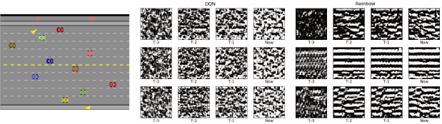
Figure 10.7
Left
: Example frame from the game Freeway (published by Activision, Inc.).
Center
and right
: Reproduced from Such et al. (2019) with permission. Input images synthe-
sized to maximally activate individual hidden units in either a DQN or Rainbow (C51)
network. Each row represents a different hidden unit; individual columns correspond to
one of the four images provided as input to the networks.
We should also expect that the type and number of predictions made by
the agent should influence the nature of the state representation. To test this
hypothesis, Such et al. (2019) studied the patterns detected by individual hidden
units in the penultimate layer of trained neural networks. In their experiments,
input images were synthesized to maximize the output of a given hidden unit
(see, e.g., Olah et al. 2018, for a discussion of how this can be done). For
example, Figure 10.7 compares the result of this process applied to networks that
either predict action-value functions (DQN) or categorical return distributions
(Rainbow (Hessel et al. 2018), a variant of C51 enhanced with additional
algorithmic components). Across multiple Atari 2600 games, Such et al. found
that making distributional predictions resulted in state representations that
better reflected the structure of the Atari 2600 game being played: for example,
identifying horizontal elements (car lanes) in the game Freeway (shown in the
figure).
Understanding how distributional reinforcement learning affects the state
representation implied by the network and how that representation affects per-
formance is an active area of research. One challenge is that deep reinforcement
learning architectures have a great deal of moving parts, many of which are
tuned by means of hyperparameters, and obtaining relevant empirical evidence
tends to be computationally demanding. In addition, changing the state repre-
sentation has a number of downstream effects on the learning process, including
changing the optimization landscape, reducing or amplifying the parameter
noise due to the use of an incremental update rule, and of course affecting the
quality of the best achievable value function approximation. Yet, the hope is that
understanding why making distributional predictions improves performance in
Draft version.
Deep Reinforcement Learning 311
domains such as the Arcade Learning Environment should shed light on the
design of more efficient deep reinforcement learning agents.
10.6 Technical Remarks
Remark 10.1.
Figure 10.1 shows that the DQN neural network is composed of
three convolutional layers, a fully connected layer, and finally a linear mapping
to the output
Q
w
(
x, a
). One appeal of neural networks is that these operations can
be composed fairly easily to add capacity to the learning algorithm or combine
different inputs: for example, the cosine embedding discussed in Section 10.3.
Let us denote the input to the network by
x ∈R
n
0
, where for simplicity of
exposition, we omit the structured nature of the input (in the case of DQN, it is
a 84
×
84
×
4 array of values; four square images). Thus, for
i ≥
0, we denote
by
n
i
∈N
the size of the “flattened” input vector to layer
i
+ 1. For
i >
0, the
i
th
layer transforms its inputs using a function
f
i
:
R
n
i−1
→R
n
i
parameterized by a
weight vector w
i
:
x
i
= f
i
(x
i−1
; w
i
), i > 0 .
In the case of DQN,
f
1
,
f
2
, and
f
3
are convolutional, while
f
4
is fully connected.
The latter is defined by a weight matrix
W
4
and bias vector
b
4
(which in our
notation are part of w
4
):
f
4
(x; w
4
) = [W
>
4
x + b
4
]
+
;
recall that for
z ∈R
, [
z
]
+
=
max
(0
, z
). In the field of deep learning, this function
is called a rectified linear transformation (ReLU; Nair and Hinton 2010).
IQN augments this network by transforming the cosine embedding
ϕ
(
τ
) with
another fully connected layer with the same number of dimensions as the output
of the last convolutional layer (n
3
):
x
3b
= f
3b
(ϕ(τ); w
3b
) .
The output of these two layers is then composed by element-wise multiplication:
x
3c
= x
3
x
3b
,
which becomes the input to the original network’s final layer:
x
4
= f
4
(x
3c
; w
4
) ,
itself linearly transformed into the quantile function estimate for (
x, a, τ
). The
reader interested in further details should consult the work of Dabney et
al. (2018a). 4
Draft version.
312 Chapter 10
10.7 Bibliographical Remarks
Beyond Atari 2600 games, the general effectiveness of deep reinforcement
learning is well established in the literature. Perhaps the most famous example
to date is AlphaGo (Silver et al. 2016), a computer Go program that learned to
play better than the world’s best Go players. Further evidence that distributional
predictions improve the performance of deep reinforcement learning agents
can be found in experiments on a variety of domains, including the cooperative
card game Hanabi (Bard et al. 2020), stratospheric balloon flight (Bellemare
et al. 2020), robotic manipulation (Bodnar et al. 2020; Cabi et al. 2020; Vecerik
et al. 2019), simulated race car control (Wurman et al. 2022), and magnetic
control of plasma (Degrave et al. 2022).
10.1.
Early reinforcement learning research has close ties with the study of
connectionist systems; see, for example, Barto et al. (1983) and Bertsekas
and Tsitsiklis (1996). Tesauro (1995) combined temporal-difference learning
with a single-layer neural network to produce TD-Gammon, a grandmaster-
level Backgammon player and early deep reinforcement learning algorithm.
Neural Fitted Q-iteration (Riedmiller 2005) implements many of the ingredients
later found in DQN, including replaying past experience (Lin 1992) and the
use of a target network; the method has been successfully used to control a
soccer-playing robot (Riedmiller et al. 2009).
The Arcade Learning Environment (Bellemare et al. 2013a), itself based
on the Stella emulator (Mott et al. 1995–2023), introduced Atari 2600 game-
playing as a challenge domain for artificial intelligence. Early results on the
Arcade Learning Environment included both reinforcement learning (Bellemare
et al. 2012a, 2012b) and planning (Bellemare et al. 2013b; Lipovetzky et
al. 2015) solutions. The DQN algorithm demonstrated the ability of deep neural
networks to effectively tackle this domain (Mnih et al. 2015). Since then, deep
reinforcement learning has been applied to produce high-performing policies
for a variety of video games and image-based control problems (e.g., Beattie
et al. 2016; Levine et al. 2016; Kempka et al. 2016; Bhonker et al. 2017; Cobbe
et al. 2020). Machado et al. (2018) study the relative performance of linear
and deep methods in the context of the Arcade Learning Environment. See
François-Lavet et al. (2018) and Arulkumaran et al. (2017) for reviews of deep
reinforcement learning and Graesser and Keng (2019) for a practical overview.
Montfort and Bogost (2009) give an excellent history of the Atari 2600 video
game console itself.
10.2–10.3.
The C51, QR-DQN, and IQN agent architectures and algorithms
were respectively introduced by Bellemare et al. (2017a), Dabney et al. (2018b),
Draft version.
Deep Reinforcement Learning 313
and Dabney et al. (2018a). Open-source implementations of these three algo-
rithms are available in the Dopamine framework (Castro et al. 2018) and the
DQN Zoo (Quan and Ostrovski 2020). The idea of implicitly parameterizing
other arguments of the prediction function has been used extensively to deal with
continuous actions; see, for example, Lillicrap et al. (2016b) and Barth-Maron
et al. (2018).
There is by now a wide variety of deep distributional reinforcement learn-
ing algorithms, many of which outperform IQN. FQF (Yang et al. 2019)
approximates the return distribution with a weighted combination of Diracs
by combining the IQN architecture with a method for selecting which values
of
τ ∈
(0
,
1) to feed into the network. MM-DQN (Nguyen et al. 2021) use an
architecture based on QR-DQN in combination with an MMD-based loss as
described in Chapter 4; typically, the Gaussian kernel has been found to provide
the best empirical performance, despite a lack of theoretical guarantees. Both
Freirich et al. (2019) and Doan et al. (2018) propose the use of generative
adversarial networks (Goodfellow et al. 2014) to model the reward distribution.
Freirich et al. also extend this approach to the case of multivariate rewards.
There are also several recent modifications to the QR-DQN architecture that
seek to address the quantile-crossing problem – namely, that the outputs of
the QR-DQN network need not satisfy the natural monotonicity constraints of
distribution quantiles. Yue et al. (2020) propose to use deep generative mod-
els combined with a postprocessing sorting step to obtain monotonic quantile
estimates. Zhou et al. (2021) parameterize the difference between successive
quantiles, rather than the quantile locations themselves, to enforce monotonic-
ity; this approach was extended by Luo et al. (2021), who directly parameterize
the quantile function via rational-quadratic splines. Developing and improving
deep distributional reinforcement learning agents continues to be an exciting
direction of research.
Several agents also incorporate a distributional loss in combination with
a variety of other deep reinforcement learning techniques. Munchausen-IQN
(Vieillard et al. 2020) combines IQN with a form of entropy regularization, and
Rainbow (Hessel et al. 2018) combines C51 with a variety of modifications
to DQN, including double Q-networks (van Hasselt et al. 2016b), prioritized
experience replay (Schaul et al. 2016), a value-advantage dueling architecture
(Wang et al. 2016), parameter noise for exploration (Fortunato et al. 2018),
and multistep returns (Sutton 1988). There has also been a wide variety of
work combining distributional RL with the actor-critic framework, typically
by modifying the critic to include distributional predictions; see, for exam-
ple, Tessler et al. (2019), Kuznetsov et al. (2020), and Duan et al. (2021) and
Nam et al. (2021).
Draft version.
314 Chapter 10
Several recent deep reinforcement learning agents have also leveraged return
distribution estimates to improve exploration. Nikolov et al. (2019) combine
C51 with information-directed exploration to obtain an agent that outperforms
IQN, as judged by human-normalized mean and median performance on Atari
2600. Mavrin et al. (2019) extract an estimate of parametric uncertainty from
distributions learned under QR-DQN and use this information to specify an
exploration bonus. Clements et al. (2020) similarly build on QR-DQN to esti-
mate both aleatoric and epistemic uncertainties and use these for exploratory
action selection. Zhang and Yao (2019) use the quantile representation learned
by QR-DQN to form a set of options, with policies that vary in their risk-
sensitivity, to improve exploration. Further use cases continue to be developed,
with Lin et al. (2019) decomposing the reward signal into independent streams,
all of which are then predicted.
10.4.
The training and evaluation protocol presented here, including the idea
of a human-normalized score, is due to Mnih et al. (2015); more generally,
Bellemare et al. (2013a) propose the use of a normalization scheme in order to
compare agents across Atari 2600 games. The sticky-actions mechanism was
proposed by Machado et al. (2018), who give evidence that a naive trajectory
optimization algorithm (see also Bellemare et al. 2015) can achieve scores
comparable to DQN when evaluated with the deterministic version of the ALE.
Our use of the interquartile mean to compare score follows the recommendations
of Agarwal et al. (2021), who also highlight reproducibility concerns when
evaluating across multiple-domain games. See also Henderson et al. (2018).
The experiments reported here were performed using the DQN Zoo (Quan and
Ostrovski 2020).
10.5.
The success of distributional reinforcement learning algorithms on large
benchmarks such as the Arcade Learning Environment is often attributed to
their use as auxiliary tasks (Jaderberg et al. 2017). Auxiliary tasks are ancillary
predictions made by the neural network that stabilize learning, shape the state
representation implied by the neural network, and improve end performance
(Lample and Chaplot 2017; Kartal et al. 2019; Agarwal et al. 2020; Laskin
et al. 2020; Guo et al. 2020; Lyle et al. 2021). Their effect on the penultimate
layer of the network is discussed more formally by Chung et al. (2018), Belle-
mare et al. (2019a), and Le Lan et al. (2022). Dabney et al. (2020a) argue that
representation learning plays a particularly acute role in deep reinforcement
learning when considering the control problem, in which the policy under eval-
uation changes over time. General value functions (GVFs) provide a language
for describing auxiliary tasks and expressing an agent’s knowledge (Sutton et
al. 2011). Schlegel et al. (2021) extend some of these ideas to the deep learning
Draft version.
Deep Reinforcement Learning 315
setting, in particular considering how GVFs are useful features in the context of
sequential prediction.
As an alternative explanation for the empirical successes of distributional
reinforcement learning, Imani and White (2018) study the effect of distributional
predictions on optimisation landscapes.
10.8 Exercises
Many of the exercises in this chapter are hands-on and open-ended in nature
and require programming or applying published learning algorithms to stan-
dard reinforcement learning domains. More generally, these exercises are
designed to give the reader some experience in performing deep reinforce-
ment learning experiments. As a starting point, we recommend that the reader
use open-source implementations of the algorithms covered in this chapter. The
Dopamine framework
78
(Castro et al. 2018) provides implementations of the
DQN, C51, QR-DQN, and IQN agents and support for the Acrobot domain.
DQN Zoo
79
(Quan and Ostrovski 2020) is a collection of open-source reference
implementations that were used to generate the results of this chapter.
Exercise 10.1.
In this exercise, you will apply deep reinforcement learning
methods to the Acrobot domain (Sutton 1996). Acrobot is a two-link pendulum
where the state gives the joint angles of the two links and their corresponding
angular velocities. Because the inputs are vectors rather than images, the DQN
agent described in this chapter must be adapted to this domain by replacing the
convolutional layers by one or multiple fully connected layers and substituting a
simple state encoding for the image preprocessing (in Dopamine, this encoding
is given by what is called Fourier features (Konidaris et al. 2011)). Of course,
the reader is encouraged to think of possible alternatives to both of these choices.
(i)
Train a DQN agent, varying the frequency at which the target network is
updated. Plot the value function over time, at the initial starting state and for
different update frequencies.
(ii)
Train a DQN agent, but now varying the size of the replay buffer. Describe
the effect of the replay buffer size on the learning algorithm in this case.
(iii)
Modify the DQN implementation to train from each transition as it is
received, rather than via the replay buffer. Compare this to the previous
results.
(iv)
Starting from an implementation of the C51 agent, implement the signed
distributional algorithm from Section 9.6. Train both C51 and the signed
78. https://github.com/google/dopamine
79. https://github.com/deepmind/dqn_zoo
Draft version.
316 Chapter 10
algorithm on Acrobot. Visualize the return-distribution function predictions
made for the same initial state, over time. Plot the average undiscounted
return obtain by either algorithm over time. Explain your findings.
(v)
Train both QR-DQN and IQN agents on Acrobot, and visualize the dis-
tributional predictions made for the same initial state. For IQN, this will
require querying the deep neural network for multiple values of
τ
. Visualize
those predictions at different points during an episode; do they behave as
expected? 4
Exercise 10.2
(*)
.
In this exercise, you will apply deep RL methods to the
MinAtar domain (Young and Tian 2019), which is a set of simplified versions
of Atari 2600 games (Asterix, Breakout, Freeway, Seaquest, Space Invaders).
(i)
Using MinAtar’s built-in human-play example, play each game for ten
episodes and log your scores. How much variability do you see between
episodes? Plot the scores versus games played; does your performance
improve over time?
(ii)
Implement a random agent that takes actions uniformly at random. Evaluate
the random agent on each MinAtar game for at least ten episodes and log
the agent’s scores for each game and episode.
(iii)
Train a C51 agent to play Breakout in MinAtar for 2 million frames
(approximately 2
.
5 hours on a GPU). Use the default hyperparameters for
the range of predicted returns (
θ
1
=
−
10 and
θ
m
= 10). Use your recorded
scores from above (for human and random players) to compute C51’s human-
normalized score. How do these compare with those reported for C51 on
the corresponding games in Atari 2600?
(iv)
Based upon your performance and that of the random agent, compute a
reasonable estimate of the maximum achievable discounted return in each
game. Train C51, again for 2 million frames, using this maximum return
to set the particle locations. Compare this agent’s performance in terms of
human-normalized score with that of the default C51 agent above. How do
they compare?
(v)
Train a QR-DQN agent on the MinAtari Breakout game, evaluating in
terms of human-normalized score. Inspecting the learned return distributions,
how do these distributions compare with those learned by C51? Do any of
the quantile estimates exceed your estimated maximal discounted return?
Why might this happen?
(vi)
Train DQN, C51, and QR-DQN agents with your preferred hyperparam-
eters, for 5 million frames with at least three seeds, on each of the five
MinAtar games. Compute the human-normalized interquartile mean score
Draft version.
Deep Reinforcement Learning 317
(HNIQM) for each method versus training steps. How do your results com-
pare with those see in Figure 10.4? Note that this exercise will require
significantly greater computational resources than others and will in general
require running multiple agents in parallel. 4
Draft version.