1
Introduction
A hallmark of intelligence is the ability to adapt behavior to reflect external
feedback. In reinforcement learning, this feedback is provided as a real-valued
quantity called the reward. Stubbing one’s toe on the dining table or forgetting
soup on the stove are situations associated with negative reward, while (for
some of us) the first cup of coffee of the day is associated with positive reward.
We are interested in agents that seek to maximize their cumulative reward –
or return – obtained from interactions with an environment. An agent maximizes
its return by making decisions that either have immediate positive consequences
or steer it into a desirable state. A particular assignment of reward to states and
decisions determines the agent’s objective. For example, in the game of Go,
the objective is represented by a positive reward for winning. Meanwhile, the
objective of keeping a helicopter in flight is represented by a per-step negative
reward (typically expressed as a cost) proportional to how much the aircraft
deviates from a desired flight path. In this case, the agent’s return is the total
cost accrued over the duration of the flight.
Often, a decision will have uncertain consequences. Travelers know that it
is almost impossible to guarantee that a trip will go as planned, even though
a three-hour layover is usually more than enough to catch a connecting flight.
Nor are all decisions equal: transiting through Chicago O’Hare may be a riskier
choice than transiting through Toronto Pearson. To model this uncertainty,
reinforcement learning introduces an element of chance to the rewards and to
the effects of the agent’s decisions on its environment. Because the return is the
sum of rewards received along the way, it too is random.
Historically, most of the field’s efforts have gone toward modeling the mean
of the random return. Doing so is useful, as it allows us to make the right
decisions: when we talk of “maximizing the cumulative reward,” we typically
mean “maximizing the expected return.” The idea has deep roots in probability,
Draft version. 1
2 Chapter 1
the law of large numbers, and subjective utility theory. In fact, most reinforce-
ment learning textbooks axiomatize the maximization of expectation. Quoting
Richard Bellman, for example:
The general idea, and this is fairly unanimously accepted, is to use some average of
the possible outcomes as a measure of the value of a policy.
This book takes the perspective that modeling the expected return alone
fails to account for many complex, interesting phenomena that arise from
interactions with one’s environment. This is evident in many of the decisions
that we make: the first rule of investment states that expected profits should
be weighed against volatility. Similarly, lottery tickets offer negative expected
returns but attract buyers with the promise of a high payoff. During a snowstorm,
relying on the average frequency at which buses arrive at a stop is likely to lead
to disappointment. More generally, hazards big and small result in a wide range
of possible returns, each with its own probability of occurrence. These returns
and their probabilities can be collectively described by a return distribution, our
main object of study.
1.1 Why Distributional Reinforcement Learning?
Just as a color photograph conveys more information about a scene than a
black and white photograph, the return distribution contains more information
about the consequences of the agent’s decisions than the expected return. The
expected return is a scalar, while the return distribution is infinite-dimensional;
it is possible to compute the expectation of the return from its distribution, but
not the other way around (to continue the analogy, one cannot recover hue from
luminance).
By considering the return distribution, rather than just the expected return,
we gain a fresh perspective on the fundamental problems of reinforcement
learning. This includes understanding of how optimal decisions should be
made, methods for creating effective representations of an agent’s state, and
the consequences of interacting with other learning agents. In fact, many of the
tools we develop here are useful beyond reinforcement learning and decision-
making. We call the process of computing return distributions distributional
dynamic programming. Incremental algorithms for learning return distributions,
such as quantile temporal-difference learning (Chapter 6), are likely to find uses
wherever probabilities need to be estimated.
Throughout this book, we will encounter many examples in which we use the
tools of distributional reinforcement learning to characterize the consequences
of the agent’s choices. This is a modeling decision, rather than a reflection of
some underlying truth about these examples. From a theoretical perspective,
Draft version.
Introduction 3
check raise
fold call
-1
+
1
+
1
+
1
+
1
+
2
+
2
+
2
+
1
+
1
+
1
+
1
+
1
+
2
+
2
+
2
-2
-2
-2 -2 -2
-2
-1
-1 -1 -1-1 -1 -1
-1
ante
ante
1.raise
2.call
win (+2)
loss (-2)
(a) (b)
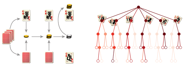
Figure 1.1
(
a
) In Kuhn poker, each player is dealt one card and then bets on whether they hold the
highest card. The diagram depicts one particular play through; the house’s card (bottom)
is hidden until betting is over. (
b
) A game tree with all possible states shaded according
to their frequency of occurrence in our example. Leaf nodes depict immediate gains and
losses, which we equate with different values of the received reward.
justifying our use of the distributional model requires us to make a number of
probabilistic assumptions. These include the notion that the random nature of
the interactions is intrinsically irreducible (what is sometimes called aleatoric
uncertainty) and unchanging. As we encounter these examples, the reader is
invited to reflect on these assumptions and their effect on the learning process.
Furthermore, there are many situations in which such assumptions do not
completely hold but where distributional reinforcement learning still provides
a rich picture of how the environment operates. For example, an environment
may appear random because some parts of it are not described to the agent (it
is said to be partially observable) or because the environment changes over
the course of the agent’s interactions with it (multiagent learning, the topic
of Section 11.1, is an example of this). Changes in the agent itself, such as
a change in behavior, also introduce nonstationarity in the observed data. In
practice, we have found that the return distributions are a valuable reflection
of the underlying phenomena, even when there is no aleatoric uncertainty at
play. Put another way, the usefulness of distributional reinforcement learning
methods does not end with the theorems that characterize them.
1.2 An Example: Kuhn Poker
Kuhn poker is a simplified variant of the well-known card game. It is played
with three cards of a single suit (jack, queen, and king) and over a single round
of betting, as depicted in Figure 1.1a. Each player is dealt one card and must
first bet a fixed ante, which for the purpose of this example we will take to be
£1. After looking at their card, the first player decides whether to raise, which
Draft version.
4 Chapter 1
Probability
Winnings
Probability
Winnings
Probability
Winnings
Probability
Winnings
10 5 0 5 10
0.0
0.2
0.4
0.6
0.8
10 5 0 5 10
0.0
0.1
0.2
0.3
10 5 0 5 10
0.0
0.1
0.2
0.3
10 5 0 5 10
0.0
0.1
0.2
0.3
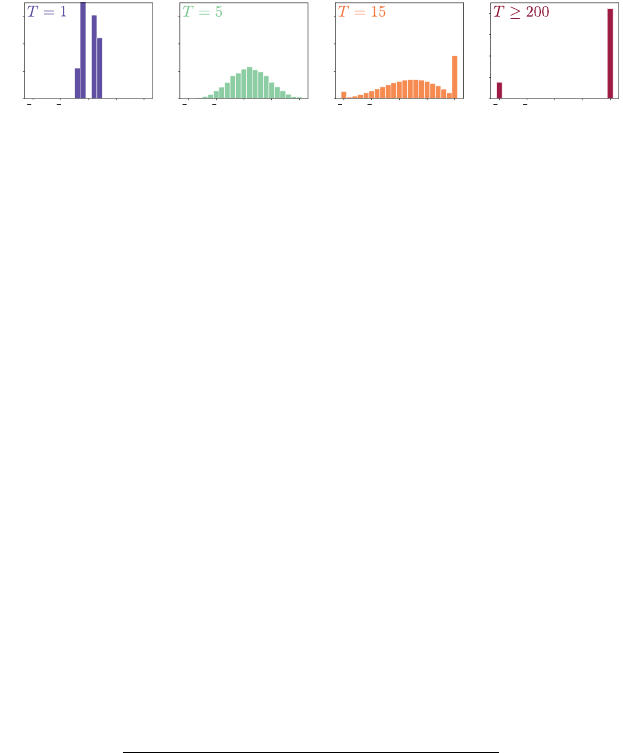
Figure 1.2
Distribution over winnings for the player after playing
T
rounds. For
T
= 1, this corre-
sponds to the distribution of immediate gains and losses. For
T
= 5, we see a single mode
appear roughly centered on the expected winnings. For larger
T
, two additional modes
appear, one in which the agent goes bankrupt and one where the player has successfully
doubled their stake. As T →∞, only these two outcomes have nonzero probability.
doubles their bet, or check. In response to a raise, the second player can call
and match the new bet or fold and lose their £1 ante. If the first player chooses
to check instead (keep the bet as-is), the option to raise is given to the second
player, symmetrically. If neither player folded, the player with the higher card
wins the pot (£1 or £2, depending on whether the ante was raised). Figure 1.1b
visualizes a single play of the game as a fifty-five-state game tree.
Consider a player who begins with £10 and plays a total of up to
T
hands
of Kuhn poker, stopping early if they go bankrupt or double their initial stake.
To keep things simple, we assume that this player always goes first and that
their opponent, the house, makes decisions uniformly at random. The player’s
strategy depends on the card they are dealt and also incorporates an element of
randomness. There are two situations in which a choice must be made: whether
to raise or check at first and whether to call or fold when the other player raises.
The following table of probabilities describes a concrete strategy as a function
of the player’s dealt card:
Holding a ... Jack Queen King
Probability of raising
1
/3 0 1
Probability of calling 0
2
/3 1
If we associate a positive and negative reward with each round’s gains or losses,
then the agent’s random return corresponds to their total winnings at the end of
the T rounds and ranges from −10 to 10.
How likely is the player to go bankrupt? How long does it take before the
player is more likely to be ahead than not? What is the mean and variance of the
player’s winnings after
T
= 15 hands have been played? These three questions
(and more) can be answered by using distributional dynamic programming
to determine the distribution of returns obtained after
T
rounds. Figure 1.2
Draft version.
Introduction 5
shows the distribution of winnings (change in money held by the player) as a
function of
T
. After the first round (
T
= 1), the most likely outcome is to have
lost £1, but the expected reward is positive. Consequently, over time, the player
is likely to be able to achieve their objective. By the fifteenth round, the player is
much more likely to have doubled their money than to have gone broke, with a
bell-shaped distribution of values in between. If the game is allowed to continue
until the end, the player has either gone bankrupt or doubled their stake. In our
example, the probability that the player comes out a winner is approximately
85 percent.
1.3 How Is Distributional Reinforcement Learning Different?
In reinforcement learning, the value function describes the expected return
that one would counterfactually obtain from beginning in any given state. It is
reasonable to say that its fundamental object of interest – the expected return
– is a scalar and that algorithms that operate on value functions operate on
collections of scalars (one per state). On the other hand, the fundamental object
of distributional reinforcement learning is a probability distribution over returns:
the return distribution. The return distribution characterizes the probability of
different returns that can be obtained as an agent interacts with its environment
from a given state. Distributional reinforcement learning algorithms operate on
collections of probability distributions that we call return-distribution functions
(or simply return functions).
More than a simple type substitution, going from scalars to probability distri-
butions results in changes across the spectrum of reinforcement learning topics.
In distributional reinforcement learning, equations relating scalars become equa-
tions relating random variables. For example, the Bellman equation states that
the expected return at a state
x
, denoted
V
π
(
x
), equals the expectation of the
immediate reward R, plus the discounted expected return at the next state X
0
:
V
π
(x) = E
π
R + γV
π
(X
0
) | X = x] .
Here
π
is the agent’s policy – a description of how it chooses actions in different
states. By contrast, the distributional Bellman equation states that the random
return at a state
x
, denoted
G
π
(
x
), is itself related to the random immediate
reward and the random next-state return according to a distributional equation:
1
G
π
(x)
D
= R + γG
π
(X
0
) , X = x .
1. Later we will consider a form that equates probability distributions directly.
Draft version.
6 Chapter 1
In this case,
G
π
(
x
),
R
,
X
0
, and
G
π
(
X
0
) are random variables, and the superscript
D
indicates equality between their distributions. Correctly interpreting the distri-
butional Bellman equation requires identifying the dependency between random
variables, in particular between
R
and
X
0
. It also requires understanding how
discounting affects the probability distribution of
G
π
(
x
) and how to manipulate
the collection of random variables G
π
implied by the definition.
Another change concerns how we quantify the behavior of learning algo-
rithms and how we measure the quality of an agent’s predictions. Because
value functions are real-valued vectors, the distance between a value function
estimate and the desired expected return is measured as the absolute difference
between those two quantities. On the other hand, when analyzing a distribu-
tional reinforcement learning algorithm, we must instead measure the distance
between probability distributions using a probability metric. As we will see,
some probability metrics are better suited to distributional reinforcement learn-
ing than others, but no single metric can be identified as the “natural” metric
for comparing return distributions.
Implementing distributional reinforcement learning algorithms also poses
some concrete computational challenges. In general, the return distribution
is supported on a range of possible returns, and its shape can be quite com-
plex. To represent this distribution with a finite number of parameters, some
approximation is necessary; the practitioner is faced with a variety of choices
and trade-offs. One approach is to discretize the support of the distribution
uniformly and assign a variable probability to each interval, what we call the
categorical representation. Another is to represent the distribution using a finite
number of uniformly weighted particles whose locations are parameterized,
called the quantile representation. In practice and in theory, we find that the
choice of distribution representation impacts the quality of the return function
approximation and also the ease with which it can be computed.
Learning return distributions from sampled experience is also more challeng-
ing than learning to predict expected returns. The issue is particularly acute
when learning proceeds by bootstrapping: that is, when the return function
estimate at one state is learned on the basis of the estimate at successor states.
When the return function estimates are defined by a deep neural network, as is
common in practice, one must also take care in choosing a loss function that is
compatible with a stochastic gradient descent scheme.
For an agent that only knows about expected returns, it is natural (almost
necessary) to define optimal behavior in terms of maximizing this quantity.
The Q-learning algorithm, which performs credit assignment by maximizing
over state-action values, learns a policy with exactly this objective in mind.
Knowledge of the return function, however, allows us to define behaviors
Draft version.
Introduction 7
that depend on the full distributions of returns – what is called risk-sensitive
reinforcement learning. For example, it may be desirable to act so as to avoid
states that carry a high probability of failure or penalize decisions that have
high variance. In many circumstances, distributional reinforcement learning
enables behavior that is more robust to variations and, perhaps, better suited to
real-world applications.
1.4 Intended Audience and Organization
This book is intended for advanced undergraduates, graduate students, and
researchers who have some exposure to reinforcement learning and are inter-
ested in understanding its distributional counterpart. We present core ideas from
classical reinforcement learning as they are needed to contextualize distribu-
tional topics but often omit longer discussions and a presentation of specialized
methods in order to keep the exposition concise. The reader wishing a more
in-depth review of classical reinforcement learning is invited to consult one
of the literature’s many excellent books on the topic, including Bertsekas and
Tsitsiklis (1996), Szepesvári (2010), Bertsekas (2012), Puterman (2014), Sutton
and Barto (2018), and Meyn (2022).
Already, an exhaustive treatment of distributional reinforcement learning
would require a substantially larger book. Instead, here we emphasize key
concepts and challenges of working with return distributions, in a mathematical
language that aims to be both technically correct but also easily applied. Our
choice of topics is driven by practical considerations (such as scalability in
terms of available computational resources), a topic’s relative maturity, and our
own domains of expertise. In particular, this book contains only one chapter
about what is commonly called the control problem and focuses on dynamic
programming and temporal-difference algorithms over Monte Carlo methods.
Where appropriate, in the bibliographical remarks, we provide references on
these omitted topics. In general, we chose to include proofs when they pertain
to major results in the chapter or are instructive in their own right. We defer the
proof of a number of smaller results to exercises.
Each chapter of this book is structured like a hiking trail.
2
The first sections
(the “foothills”) introduce a concept from classical reinforcement learning and
extend it to the distributional setting. Here, a knowledge of undergraduate-level
probability theory and computer science usually suffices. Later sections (the
“incline”) dive into more technical points: for example, a proof of convergence
or more complex algorithms. These may be skipped without affecting the
2. Based on one of the author’s experience hiking around Banff, Canada.
Draft version.
8 Chapter 1
reader’s understanding of the fundamentals of distributional reinforcement
learning. Finally, most chapters end on a few additional results or remarks that
are interesting yet easily omitted (the “side trail”). These are indicated by an
asterisk (
∗
). For the latter part of the chapter’s journey, the reader may wish to
come equipped with tools from advanced probability theory; our own references
are Billingsley (2012) and Williams (1991).
The book is divided into three parts. The first part introduces the building
blocks of distributional reinforcement learning. We begin by introducing our
fundamental objects of study, the return distribution and the distributional
Bellman equation (Chapter 2). Chapter 3 then introduces categorical temporal-
difference learning, a simple algorithm for learning return distributions. By
the end of Chapter 3, the reader should understand the basic principles of
distributional reinforcement learning and be able to use them in simple practical
settings.
The second part develops the theory of distributional reinforcement learn-
ing. Chapter 4 introduces a language for measuring distances between return
distributions and operators for transforming with these distributions. Chapter 5
introduces the notion of a probability representation, needed to implement
distributional reinforcement learning; it subsequently considers the problem of
computing and approximating return distributions using such representations,
introducing the framework of distributional dynamic programming. Chapter 6
studies how return distributions can be learned from samples and in a incre-
mental fashion, giving a formal construction of categorical temporal-difference
learning as well as other algorithms such as quantile temporal-difference learn-
ing. Chapter 7 extends these ideas to the setting of optimal decision-making
(also called the control setting). Finally, Chapter 8 introduces a different perspec-
tive on distributional reinforcement learning based on the notion of statistical
functionals. By the end of the second part, the reader should understand the
challenges that arise when designing distributional reinforcement learning
algorithms and the available tools to address these challenges.
The third and final part develops distributional reinforcement learning for
practical scenarios. Chapter 9 reviews the principles of linear value function
approximation and extends these ideas to the distributional setting. Chapter 10
discusses how to combine distributional methods with deep neural networks
to obtain algorithms for deep reinforcement learning. Chapter 11 discusses the
emerging use of distributional reinforcement learning in two further domains of
research (multiagent learning and neuroscience) and concludes.
Code for examples and exercises, as well as standard implementations of the
algorithms presented here, can be found at http://distributional-rl.org.
Draft version.